
My FLOPS 2022 keynote talk: “Adventures in Building Reliable Distributed Systems with Liquid Haskell”
Back in May, I gave the opening keynote (my first keynote talk!) at the FLOPS 2022 conference. I talked about the work we’ve been doing in my group on using Liquid Haskell for verifying the correctness of distributed systems.
Here’s a pseudo-transcript1 of my FLOPS talk. Some of the slides are included below, and I’ve posted the full set of slides as well.
Good morning
Good morning, FLOPS! I’m Lindsey Kuper. I’m an assistant professor at UC Santa Cruz.
Thank you very much to Atsushi and Michael and to the entire FLOPS organizing team for inviting me to speak at FLOPS and for their work organizing this event. On a personal note, FLOPS was the very first conference that I ever had a paper rejected from, way back in 2010 as a beginning grad student. So I feel particularly honored to have been asked to give this talk today.
This talk will be about something I’ve been very excited about recently, which is the potential of using modern language-integrated verification tools to help us build distributed systems that are guaranteed to work like they’re supposed to, and for those guarantees to apply not just to models, but to real, running code.
In the beginning part of this talk, I’ll explain what I mean by “distributed systems” and what kinds of specific challenges they present. Then I’ll briefly introduce the Liquid Haskell language-integrated verification system. Finally, the adventures: I’ll share some highlights of two projects in this space that my students and collaborators and I have been working on.
So, let’s start by talking about distributed systems!
What’s a distributed system?
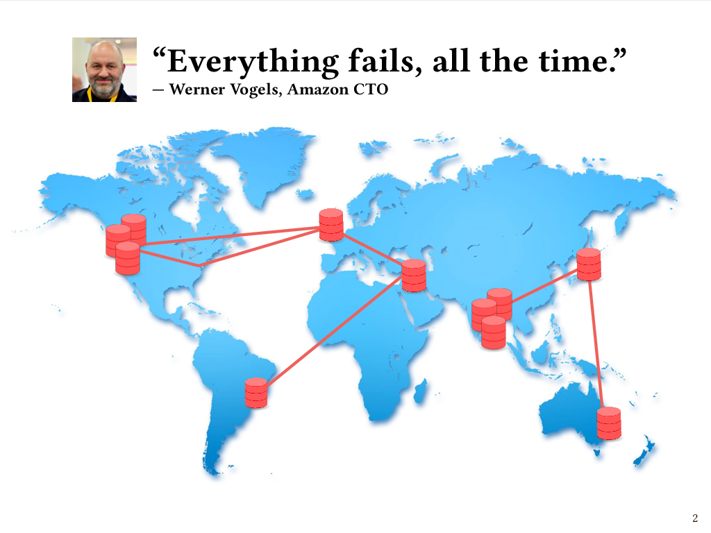
Imagine some number of independent machines that communicate by passing messages to one another over a network. They could be close or far apart, but we’re especially interested in so-called geo-distributed systems where that network may span the whole planet. For example, the nodes in this graph roughly correspond to the locations of some of Amazon’s data centers. It’s at this larger “planet-scale” that some of the most interesting and challenging issues arise.
Many of those issues have to do with failure, and the need to keep operating in the presence of partial failure of a system. Amazon had a very colorful description of this in their SOSP 2007 paper on the Dynamo data storage system: “Customers should be able to add items to their shopping carts even if disks are failing, network routes are flapping, or data centers are being destroyed by tornadoes.” (I happen to be from Iowa, in the midwestern United States, so tornadoes were very real to me growing up, but feel free to substitute any natural disaster of your choosing.)
So, not only can network connections fail, but nodes in this network can fail as well, due to tornadoes or whatever other reason. And it’s important for the system to continue to operate and respond to requests even during a failure, because, in the pithy words of Werner Vogels, “Everything fails, all the time.”
So, this problem of partial failure, and needing to continue to operate in the presence of partial failure, is in many ways the defining characteristic of distributed systems.
The speed of light is slow
But in geo-distributed systems we have another fundamental problem, which is that the speed of light is slow!
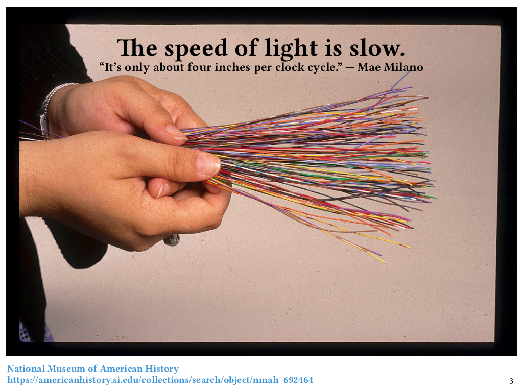
This is a bundle of pieces of wire, each about 30 centimeters long. Grace Hopper famously distributed these at her lectures to demonstrate the distance that an electrical signal can travel in one nanosecond. These were some of the actual pieces of wire she handed out; they’re at the Smithsonian now.
So, the speed of light is slow! It only goes about 30 centimeters in a nanosecond. Or, as my friend Mae Milano puts it, it’s only about four inches per clock cycle.
So, if we’re talking about machines that might be on opposite sides of the world from each other, that’s a lot of clock cycles that can go by between when a message is sent and when it arrives, even under ideal conditions.
Replication
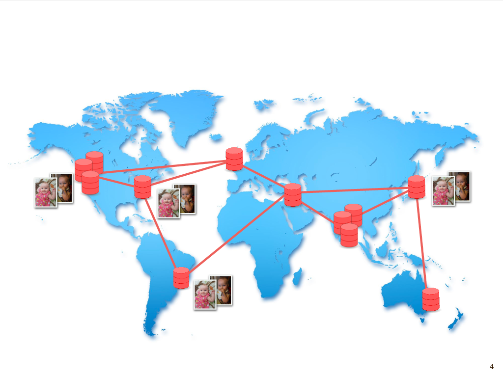
So, whether we’re talking about failure – disks failing, cosmic rays, network connections being taken out by backhoes, data centers being taken out by tornadoes – or just the more mundane but unavoidable issue of long latency between machines that are far apart, one way to mitigate these challenges is to have data that’s replicated across a number of physical locations. This helps ensure the availability of data – in other words helps ensure that every request gets a meaningful response.
If I have data that I both don’t want to lose and that I want to make sure remains available, whether it’s baby pictures of my daughter or any other data that I may care about, I’m going to store multiple replicas of that data both within data centers and across different data centers.
This is done for reasons of, again, fault tolerance – the more copies you have, the less likely it is you’ll lose it – as well as data locality to minimize latency – we want a copy of the data to be close to whoever’s trying to access it – and reasons of throughput, too: if you have multiple copies of data, then in principle you can serve more clients who are trying to simultaneously access it. But, while having multiple copies is essential for all of these reasons, it introduces the new problem of having to keep the replicas consistent with each other, particularly in a network where we have can have arbitrarily long latency between replicas, due to network partitions.
Consistency
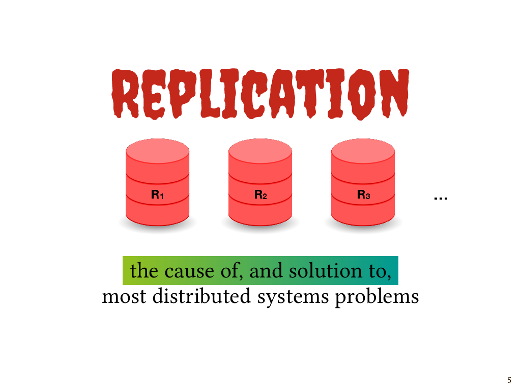
So, as I tell the undergrads who take my distributed systems course, replication is both the cause of, and solution to, most distributed systems problems. We have to replicate data, but then we have to keep those replicas consistent with one another.
Now, we know that trying to keep geo-distributed replicas perfectly consistent at all times is a fool’s errand. A classic impossibility result tells us that the only way to accomplish perfect consistency in the presence of network partitions is to compromise on the availability of our data. Since network partitions are an inevitability when working with geo-distributed data, we often choose to design systems in ways that permit clients to observe certain kinds of disagreement among replicas, in the interest of prioritizing availability.
If we’re going to allow certain kinds of disagreement among replicas, then we need a way of specifying a policy that tells us in what ways replicas are allowed to disagree, and under what circumstances they are allowed to disagree, and under what circumstances they must agree. Let’s look at a couple examples of these consistency policies, and some ways in which they can be violated.
Strong convergence
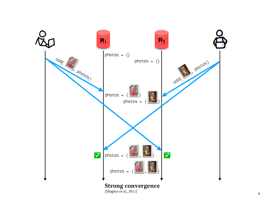
One of the properties of interest is called strong convergence. This says that if replicas have received the same set of updates – in any order – then those replicas have equivalent state. For instance, let’s say that my partner and I are both updating our shared photo album of pictures of our daughter, called photos. I add one photo, which makes it first to replica R1 and, a little while later, to replica R2. Meanwhile, my partner adds a different photo, which makes it first to R2 and, later, to R1. Although the replicas receive the updates in opposite orders, their states agree at the end. So, this execution enjoys the property strong convergence.
In this example, it’s pretty obvious that this is the case, since our replicated data structure is a set, and these two additions of elements to the set commute with each other.
Ensuring strong convergence
In general, however, we have to carefully design the interface of our data structures to ensure that strong convergence holds in every execution.
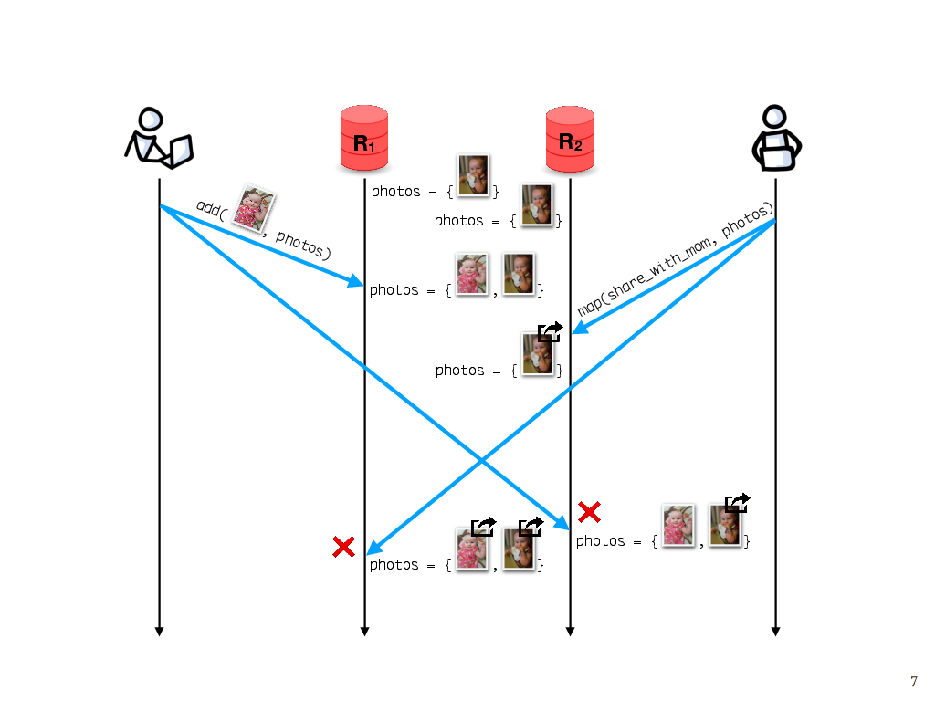
For instance, here’s a different execution that isn’t strongly convergent. Say we start with both replicas having the same photo album containing one photo. As before, I add one photo. Let’s suppose that my photo makes it first to R1. Meanwhile, let’s say that our photo application offers a share_with_mom operation that takes a photo as its argument. My partner wants to share the photos with his mom, so he tries to map the share_with_mom operation over everything in the photo album.
The map operation makes it to R2 first, and gets applied to everything in the photo album, which at that point is just one photo. But later when the photo that I added arrives, it wasn’t part of the set at the time the map operation ran, so according to replica R2, it isn’t shared with my mother-in-law. Meanwhile, replica R1 receives the map operation second and maps over both photos, so both photos get shared. These operations unfortunately don’t commute with each other, and so, if this map operation is part of the interface that our photo album provides, then strong convergence wouldn’t hold for every execution.
One way to fix this is to carefully design the data structure’s interface in a way that ensures that all operations on it do commute. Data structures with this behavior are known as conflict-free replicated data types or CRDTs, and they often work by playing clever tricks to make operations commute when they otherwise wouldn’t, or leveraging assumptions about the order in which operations are applied. New CRDT designs are an active area of research. As the designs of these data structures get more complex, they motivate the need for mechanically verified implementations that are guaranteed to converge in all possible executions.
We’ll come back to that later, but before we do, let’s look at a different kind of consistency issue.
Causal delivery
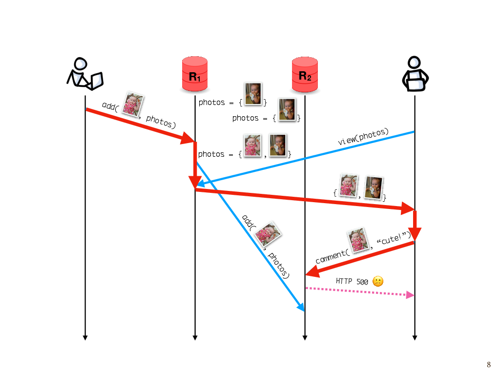
Let’s say, once again, that I add a photo to the album. I happen to communicate with replica R1, and R1 asynchronously sends the update to R2. Later, my partner comes along to look at the photos. He sees my update, because he happens to talk to the same replica as the one on which the update was made. But suppose he tries to leave a comment after that, and unfortunately, that write goes to R2, which hasn’t gotten the photo yet. Because the photo isn’t there yet, the replica can’t attach the comment to it.
This would probably manifest as some sort of inscrutable error message, like “Sorry, something went wrong. Try again.” You’ve probably seen this sort of thing before.
To see what went wrong here, we have to consider the causality of events. My partner attempted to leave a comment on the photo because he saw the photo in a response from the server. And that happened because of the previous add operation. So, this add operation is part of the causal history of the attempted comment, which we can see by following these messages forward through time and seeing that the comment operation is reachable from the add operation. But at the time the attempted comment happened, this replica hasn’t found out about this add event that’s in its causal history. So this is a violation of what’s known as causal consistency.
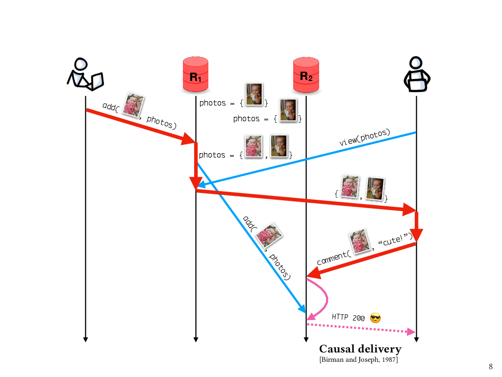
One way to fix this is to use a mechanism that ensures messages are delivered to replicas in causal order, where the word “delivered” means actually applied to the replica’s state after having been received. A widely used approach is to attach metadata to each message that summarizes the causal history of that message – for example, a vector clock. We can use this metadata to determine the causal relationship between two messages, if there is one, and delay the delivery of a message to a given replica until every causally preceding message has been delivered. In this case, the comment message to replica R2 would be queued until the add message arrives and then the comment can be applied. Here again, I’d argue there’s a need for mechanically verified implementations, since a causal message ordering abstraction is such a useful building block of distributed systems, but a lot of systems don’t get this right. And we’ll come back to this later.
What consistency policy should we enforce?
It turns out that even knowing which policy we should enforce is nontrivial, because these consistency policies, and the properties that they specify about executions, don’t necessarily map nicely onto the invariants that we care about for a given application.
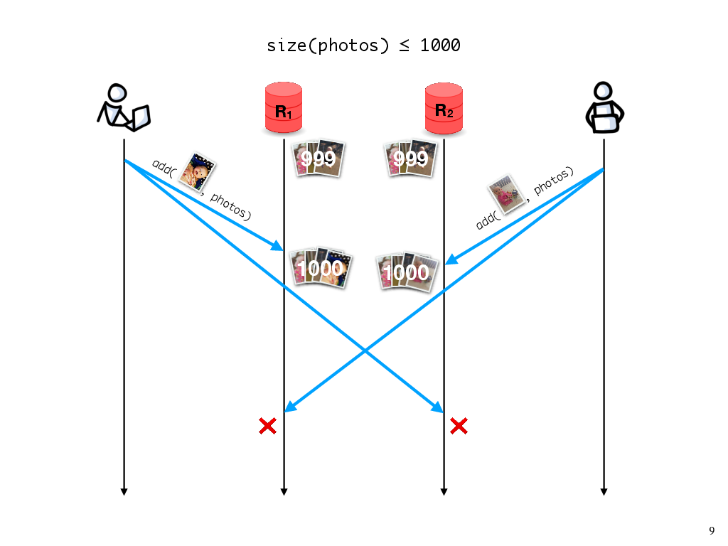
Let’s say, for instance, that my partner and I are using the free tier of a photo sharing service, which says that we can have at most 1000 photos, and otherwise we have to start paying or we risk our old photos being deleted. If we have 999 photos in the album, adding one photo should be fine; the invariant hasn’t been violated.
On the other hand, what if my partner also adds a photo concurrently? Then, when the two replicas synchronize, the invariant will be violated.
What should we do about this? If the invariant needs to be maintained, then either my update or my partner’s update would need to be rejected, which would require us to synchronize replicas every time we add a photo. In practice, we might want to avoid this synchronization until we get close to the 1000-photo limit. Furthermore, other operations, like deleting a photo, wouldn’t require the synchronization to maintain this particular invariant. In general, the need for replicas to synchronize will depend on the operation and on the application-specific invariant we need to maintain.
The application-agnostic properties that we talked about earlier, like strong convergence and causal message delivery, don’t get us all the way there, but they might get us some of the way. In fact, work on verifying these application-specific properties often rests on assumptions that properties like strong convergence or causal message delivery are already present. And we can simplify the application-level verification task (or, for that matter, just the informal reasoning about the behavior of application code) if we can rely on certain properties being true of the underlying data structures, or underneath that, the messaging layer.
The distributed consistency policy zoo
So we’ve just seen a couple examples of policies that we might want to enforce about the consistency of replicated data. Knowing that such a policy will hold for all executions requires reasoning about an often very large state space of executions, with lots of possibilities for message loss and message ordering.
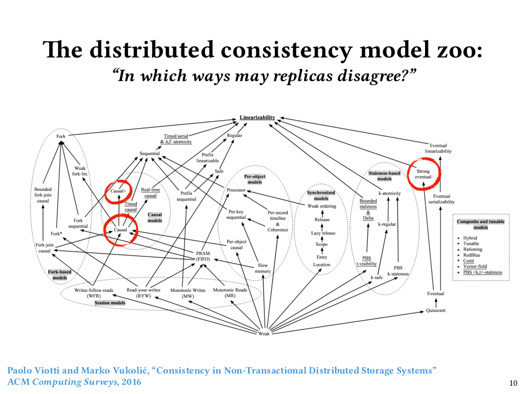
The specifications of these policies are called consistency models, and there are a lot of them. I showed this figure to my grad students a while ago, and now it haunts their dreams. It’s from a survey paper published in 2016 by Viotti and Vukolić that catalogued over fifty notions of consistency from the distributed systems literature, and ordered them by their so-called “semantic strength”. In other words, the higher up you go in this ordering of consistency models, the fewer executions are allowed, and the less disagreement among replicas is allowed. The lower you go, the more executions are allowed, and the more disagreement among replicas. And, as you can see, it’s a partial order – there are many pairs of consistency models for which neither is stronger than the other.
Just now, we looked at two points in this space. Causal consistency, which we just talked about, is over on the left. Strong convergence, which we talked about previously, does not appear on Viotti and Vukolić’s figure, although they did talk about it in their paper. If it did appear, it would have to be a lower bound of both “Strong eventual consistency” over on the right side, and “Causal+ consistency” over on the left side.
Although strong convergence doesn’t appear on the figure, I think it is a nice property to consider independently, because it’s the safety piece of strong eventual consistency. This figure is a bit bewildering, not only because this partially ordered set has so many elements, but also because some of the elements of the set lump together safety and liveness properties. But if it is bewildering, that only goes to show that even figuring out how to specify the behavior we want from distributed systems is hard (let alone actually verifying that those specifications are satisfied).
So we have two problems. One problem is making precise what policy, or combination of policies, or parts of a policy, that we want for a given application. Another problem is ensuring that no execution violates that policy. These are hard problems, and programmers shouldn’t have to tame this zoo all on their own without help. Programmers ought to have powerful, language-integrated tools for specifying the behavior they want from distributed system implementations and then ensuring that their implementations meet those specifications.
The blue-sky vision
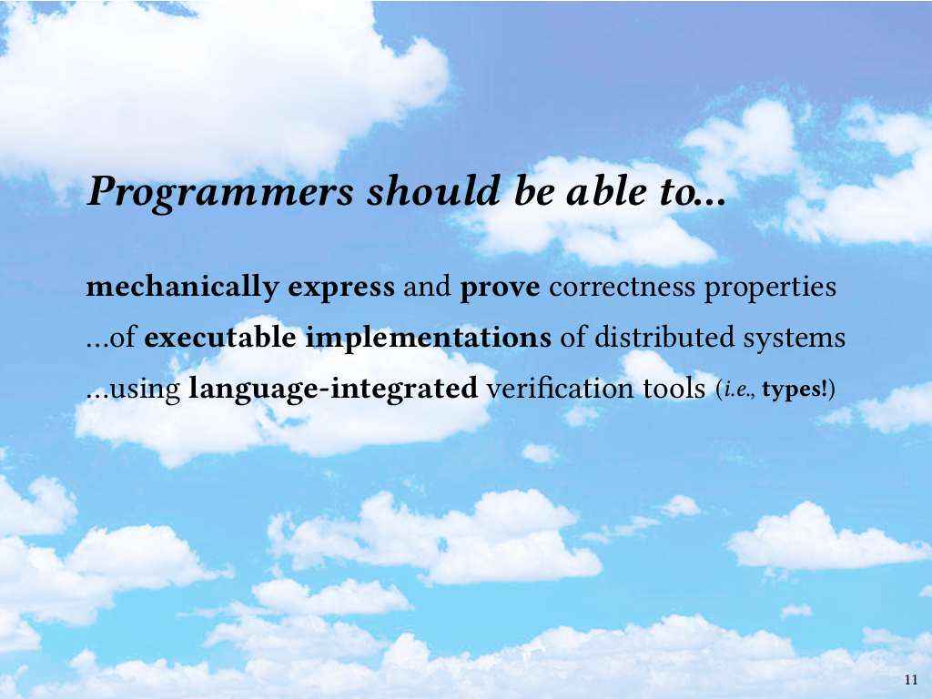
So, that’s the blue-sky vision: we want programmers to be able to mechanically specify and verify correctness properties – not just of models, but of real, executable implementations of distributed systems. Moreover, they should be able to do this using verification capabilities integrated into the same general-purpose, industrial-strength programming language that they use for implementation.
Many of us are already sold on language-integrated verification by means of expressive type systems, and that’s the approach to verification that I’m going to be talking about today.
This brings me to the next part of the talk. We’ve just talked about distributed systems and some examples of properties we might want to specify and verify; now we’ll introduce Liquid Haskell and turn to how, and indeed whether, we can use Liquid Haskell to accomplish what we want.
Refinement types
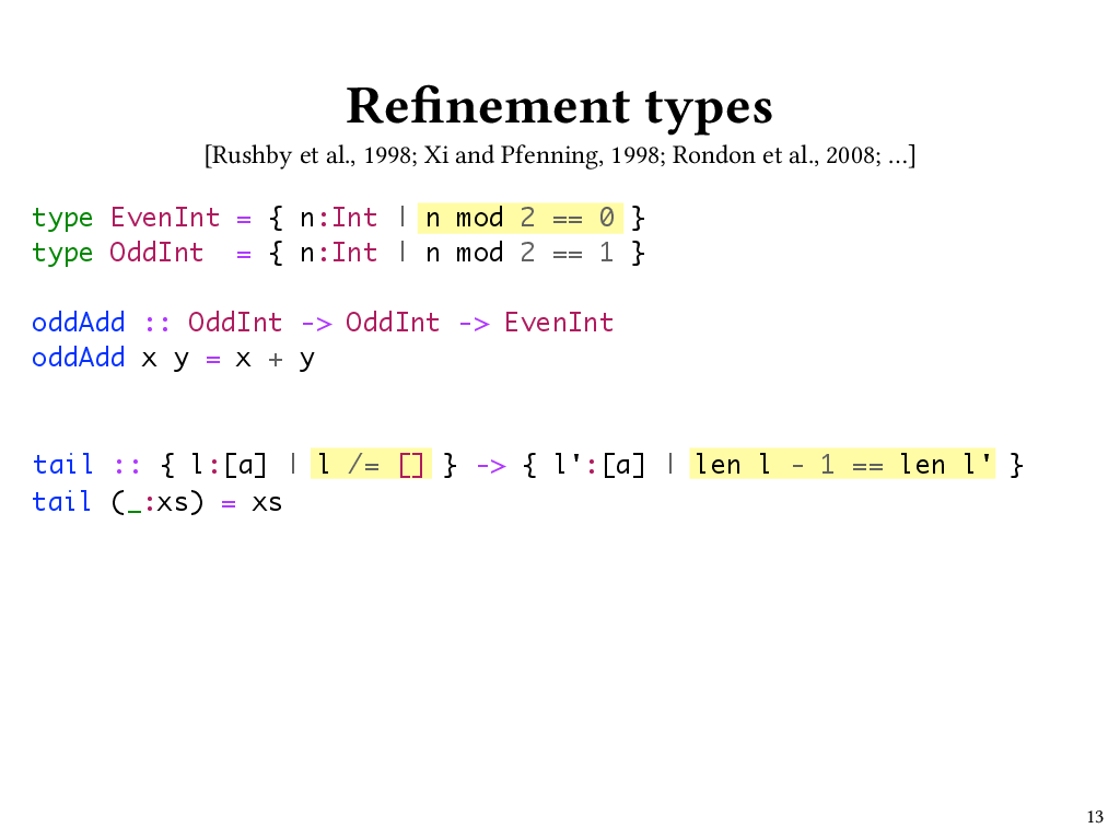
The language-integrated verification approach taken by Liquid Haskell centers around refinement types. For the purposes of this talk, I’ll define refinement types as data types that let programmers specify logical predicates that restrict, or refine, the set of values that can inhabit the type. Depending on the expressivity of the predicate language, programmers can specify rich properties using refinement types, sometimes at the expense of decidability of type checking. Liquid types, on which Liquid Haskell is based, avoid that problem by restricting the refinement predicates to an SMT-decidable logic.
Here are a couple of simple examples, which I’ve written using Liquid Haskell syntax.
For instance, we can define a type called EvenInt that refines Haskell’s built-in Int type with a refinement predicate, which I’ve highlighted here, that says that our Int has to be evenly divisible by 2.
type EvenInt = { n:Int | n mod 2 == 0 }
Likewise we could define an OddInt type with a refinement predicate that says that we get a remainder of 1 when dividing by 2.
type OddInt = { n:Int | n mod 2 == 1 }
Let’s look at how we could use these types. In Liquid Haskell I could write a function called oddAdd that takes two OddInts and returns their sum. The type of the arguments expresses the precondition that x and y will be odd, and the return type, EvenInt, expresses the postcondition that x + y will evaluate to an even number.
oddAdd :: OddInt -> OddInt -> EvenInt
oddAdd x y = x + y
Liquid Haskell automatically proves that such postconditions hold by generating verification conditions that are checked at compile time by an underlying SMT solver. If the solver finds a verification condition to be invalid, typechecking fails. For example, if the return type of oddAdd had been OddInt, then the oddAdd function would fail to type check, and Liquid Haskell would produce a type error message.
Although none of this is news to people familiar with refinement types, it’s worth pointing out that just with what we’ve seen so far, we can already do some rather useful things. For example, here’s a function called tail from the Haskell Prelude, Haskell’s standard library, which, given a list, gives everything that comes after the head of that list, which must be non-empty. If you were to call tail on an empty list, you would get an exception at run time.
tail :: [a] -> [a]
tail (_:xs) = xs
tail [] = error "oh no!"
Using refinement types, we can give tail a type that says that its input cannot be an empty list.
tail :: { l:[a] | l /= [] } -> [a]
tail (_:xs) = xs
If we do this, then we can actually get rid of the empty list case, making our code a little simpler.
Moreover, we can also add a refinement predicate to the return type of tail that will say something about the length of the list it returns; in particular, that it’s one shorter than the length of the argument list. So now tail has a postcondition that might be useful to callers of tail.
tail :: { l:[a] | xs /= [] } -> { l':[a] | len l - 1 == len l' }
So far, this is pretty much what you would expect from a refinement type system. Where I think Liquid Haskell really shines, however, is where it lets you go beyond specifying preconditions and postconditions of individual functions, and lets you verify extrinsic properties that are not specific to any particular function’s definition, using a mechanism called refinement reflection. Let’s return to our even-and-odd example to see what that might look like.
Refinement reflection
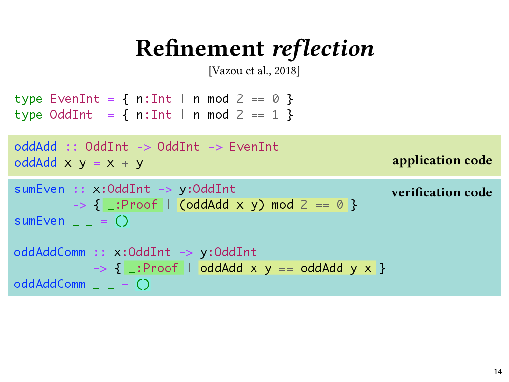
Here’s a type annotation for a function called sumEven. The type of sumEven expresses the extrinsic property that oddAdd returns an even number. In fact, sumEven is a Haskell function that returns a proof that oddAdd returns an even number.
We see that the return type of sumEven is Proof. In Liquid Haskell, this Proof type is just a type alias for Haskell’s () (unit) type. The refinement predicate that refines Proof specifies the property that we want to prove – namely, that when we call oddAdd, the result will be even. We’re able to refer to oddAdd in the refinement type of sumEven thanks to Liquid Haskell’s refinement reflection mechanism.
We can now write the body of the sumEven function: it ignores its arguments and returns () (unit). The body of sumEven doesn’t look like much – but it is an honest-to-goodness proof term! The reason it doesn’t look like much is that this particular proof – the proof that if x and y are odd, then a call to oddAdd x y will evaluate to an even number – is one that’s easy for the underlying SMT solver to carry out automatically. If that weren’t the case, then we would need to write a fancier proof term here, using the proof combinators that Liquid Haskell provides.
Now, sumEven isn’t too exciting of a property; after all, it doesn’t tell us anything that we didn’t already know from the refinement type of oddAdd. But now that we have the ability to refer to oddAdd in refinement predicates, we can do more interesting things, too. For example, I can use Liquid Haskell to prove that oddAdd is commutative. This time the refinement predicate on our return type has two calls to oddAdd, so we need a proof relating the results of multiple calls. And once again, Liquid Haskell can come up with this proof automatically. It does so in part by leveraging the underlying SMT solver’s knowledge that addition on ints is commutative.
While both of these proofs were automatic, in general, this may not be the case. Liquid Haskell programmers can specify arbitrary extrinsic properties in refinement types, and the programmer can then prove those extrinsic properties by writing programs that inhabit those refinement types, using the provided proof combinators.
So, Liquid Haskell can do more than traditional refinement types. It doesn’t just let you give more precise types to programs you were writing anyway. It also lets you use refinement type annotations as a place to specify any decidable property about your code that you might want to prove. You can then assist the SMT solver in proving that property by writing Haskell programs to inhabit those types.
I see Liquid Haskell as sitting at the intersection of SMT-based program verifiers such as Dafny, and proof assistants that leverage the Curry-Howard correspondence like Coq and Agda. A Liquid Haskell program can consist of both application code, like oddAdd (which runs at execution time, as usual) and verification code, like sumEven and oddAddComm, which are only typechecked, but, pleasantly, both of them are just Haskell programs, just with refinement types. Being based on Haskell lets programmers gradually port code from plain Haskell to Liquid Haskell, adding richer specifications to code as they go. For instance, a programmer might begin with an implementation of oddAdd with the type Int -> Int -> Int, later refine it to OddInt -> OddInt -> EvenInt, yet later prove the extrinsic properties sumEven and oddAddComm, and still later use the proofs returned by sumEven and oddAddComm as premises to prove another, more interesting extrinsic property.
A final thing to note is that unlike with a traditional proof assistant, which requires you to extract an executable implementation from the code you wrote in the proof assistant’s vernacular language, in Liquid Haskell you’re proving things directly about the code you’re going to run, so at the end, you have immediately executable verified code with no extraction step required, and hence no need to trust the extraction process.
Adventures
Now that we’ve had a taste of Liquid Haskell, let’s get on to the fun part: the adventures! In my group, we’ve been looking at how to use Liquid Haskell, and in particular how we can use this nifty refinement reflection capability, to express and prove interesting properties of implementations of distributed systems.
In particular, we’re interested in addressing two of the problems I discussed in the beginning part of the talk: first, making sure that replicated data structures are strongly convergent, and second, guaranteeing that messages are delivered at replicas in causal order. A third problem I discussed in the beginning part of the talk is this problem of guaranteeing that application-specific invariants hold, and while I won’t be talking about that one specifically, I’ll point out that one of our goals is for the results of these first two verification tasks to be usable as modular building blocks in the verification of these application-level properties. So if we’re successful, that third task will be easier.
Verified strong convergence of CRDTs
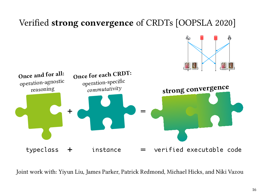
So first, verification of strong convergence of replicated data structures. This was joint work with collaborators Yiyun Liu, James Parker, Michael Hicks, and Niki Vazou, and my PhD student, Patrick Redmond. Recall from before that strong convergence means that if replicas have applied the same set of update operations, in any order, then they have equivalent state. Data structures that give you this property are called conflict-free replicated data types, or CRDTs.
Like we saw before, the strong convergence of a replicated data structure depends on the commutativity of the operations on that data structure. This depends on which operations the data structure provides. However, once you have that commutativity proof, the rest of the reasoning to get strong convergence is independent of the specifics of the particular replicated data structure.
We able to leverage this independence by stating and proving the strong convergence property at the level of a generic CRDT interface in Liquid Haskell, and then plugging in a data-structure-specific commutativity proof for each individual CRDT we wanted to verify.
In Haskell, those generic interfaces are called typeclasses, and being able to do this proof in this modular fashion required extending Liquid Haskell to add the ability to state and prove properties at the typeclass level. This was actually a huge challenge, because Liquid Haskell operates at an intermediate level of Haskell code, after typeclasses have been compiled away. My collaborators extended Liquid Haskell to support typeclasses, which required an overhaul of Liquid Haskell and came with its own interesting challenges, and you can read all about that in our OOPSLA ‘20 paper.
Once it was possible to state and prove properties of typeclasses in Liquid Haskell, it meant that an operation-agnostic proof at the CRDT typeclass level could be combined with a operation-specific commutativity proof at the individual CRDT level to get a complete proof of strong convergence for that CRDT.
Let’s take a closer look at the property we needed to prove at the typeclass level, and how we expressed it in Liquid Haskell.
A verified CRDT typeclass
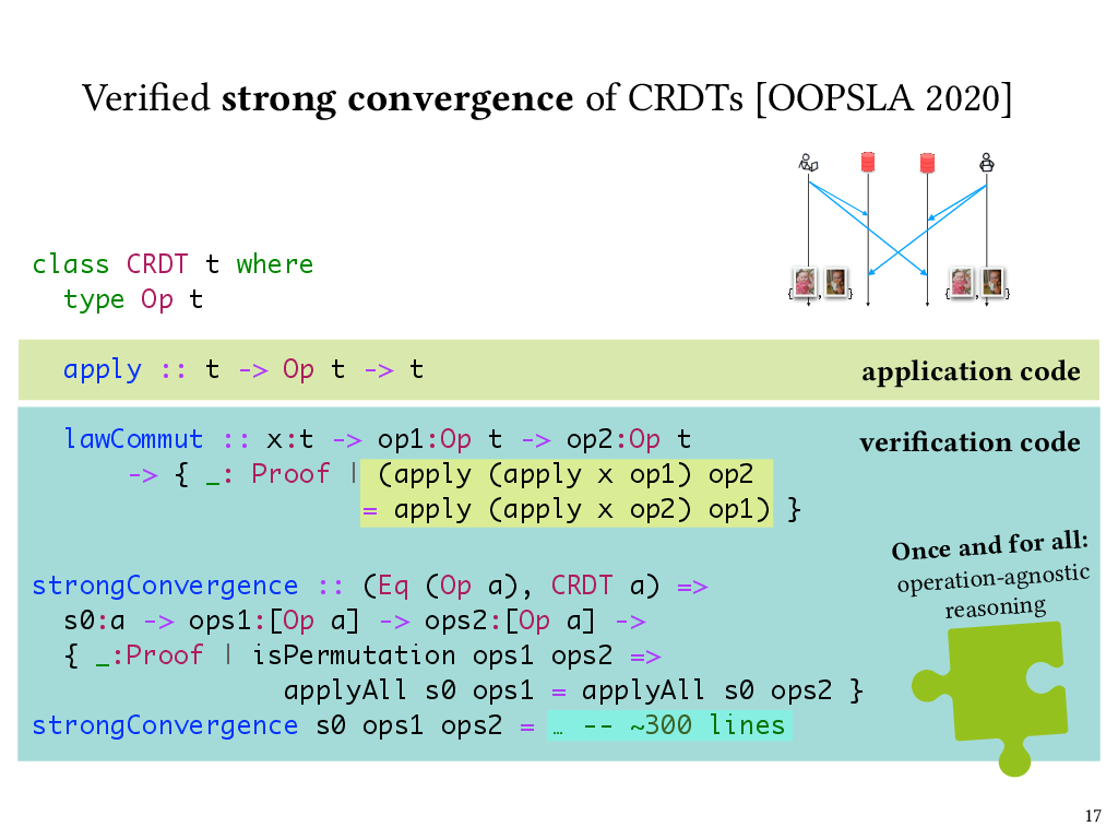
So, here’s a Liquid Haskell typeclass for CRDTs. Each instance of the typeclass has an associated Op type that specifies the operations that can update the CRDT’s state. The apply method takes a state, runs the given operation on it, and returns the updated state.
The type of lawCommut specifies the property that operations must commute, and implementors of individual CRDT instances need to provide such a commutativity proof.
What I’m showing here is a simplified version of the CRDT typeclass that leaves out some subtlety in our actual implementation. In particular, it’s not actually the case that all operations must commute; instead there is a notion of “compatible” operations that is CRDT-specific, and it’s in fact only compatible operations that must be commutative, because the design of the CRDT rules out incompatible operations from being applied concurrently. Furthermore, some operations can only be applied when the CRDT is in a given state. For the simplest CRDTs, like a grow-only counter, all operations would be compatible with each other and are always applicable, whereas for more sophisticated CRDTs, this isn’t the case. And you can find more details on this notion of compatibility in our paper.
Once we were able to define the CRDT typeclass this way, we were able to express a strong convergence property at the level of the typeclass. Here’s the statement of the strongConvergence property in Liquid Haskell. This is again simplified from the real thing, but captures the key idea, which is that if two lists of operations are permutations of one another, then applying either one to the same input CRDT state will produce the same output state. The proof of this property is about 300 lines of Liquid Haskell code. It’s by induction over the operation lists and makes use of the operation commutativity proof supplied by CRDT instances. However, the strongConvergence proof is independent of any particular CRDT instance, and thus applies to all of them.
I made a distinction earlier between application code and verification code, and we can see that here as well. The apply function is actually used at run time in the implementation of CRDTs. The lawCommut function and the strongConvergence function never run at runtime, so they’re verification code. But we can see from the refinement type of lawCommut that it’s a proof about the behavior of apply, and it’s because of Liquid Haskell’s refinement reflection that it’s possible to refer to apply in lawCommut’s type. Finally, lawCommut is called as a function, or in other words, used as a lemma, in the body of strongConvergence, which isn’t shown here because it’s too long.
Verified CRDT instances
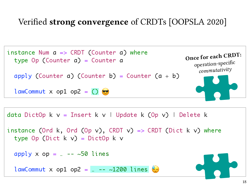
Now, how easy is it for CRDT instances to supply this operation commutativity proof lawCommut? It depends on the complexity of the CRDT. Here are a couple of examples.
One of the simplest CRDTs is a counter that can only grow. Operations on this counter are just numbers, and the state of the CRDT is their sum. For this CRDT, Liquid Haskell can carry out the commutativity proof automatically, just like it could for the proof that addition is commutative that I showed a while ago.
On the other hand, here’s a fancier CRDT: a dictionary that supports insert, update, and delete operations on key-value pairs, and where the values themselves are of CRDT type. For this CRDT, the commutativity proof took over a thousand lines of code.
Complexity in the commutativity proofs is the result of complexity in the CRDTs’ implementation. For instance, for this dictionary CRDT, I’ve elided the implementation of the apply function, but it’s a bit hairy. For example, if it receives update operations for a key that hasn’t been inserted yet, it stores those update operations in a buffer of pending operations, and then applies them as soon as the relevant insertion happens.
It’s worth pointing out that this implementation complexity is necessary because these CRDTs are designed in a way that requires very little in terms of ordering guarantees from the underlying messaging layer. That’s why it’s possible for a replica to receive update operations for a key that hasn’t yet reached that replica. While this does means that we can potentially use our CRDTs in more settings, it makes for a more strenuous verification effort for nontrivial CRDTs.
Although we already have some modularity in the way that we separate our CRDT-agnostic strong convergence proof from CRDT-specific commutativity proofs, this strenuous verification effort suggests that an even more modular approach that separates lower-level message delivery concerns from higher-level data structure semantics is called for. That idea will lead us into the second and final project that I’ll discuss in this talk.
Back to causal delivery
Let’s recap the example we saw earlier to motivate the need for causal message delivery. In this example, I’ve updated a shared photo album with a new photo, and my partner sees it, but when he tries to leave a comment on the new photo, he communicates with a replica that hasn’t gotten the update yet. As we discussed, this is a violation of causal order of messages: his comment causally depends on my previous photo add operation.
One way to solve this kind of problem is to have replicas keep track of metadata representing how many messages they’ve delivered from each other, and for messages to carry metadata representing their causal dependencies, and not deliver a message at a replica until its dependencies have been satisfied. For instance, the response from replica 1 to my partner could carry a vector clock that indicates that replica 1 is aware of one message delivery, and this vector clock metadata could be threaded through in the next request from the client. When the request arrives at replica 2, replica 2 can check the vector clock, compare it to its own clock, determine if the message is deliverable, and if necessary, queue the message until the causally preceding message has been received and delivered.
Specifying causal delivery
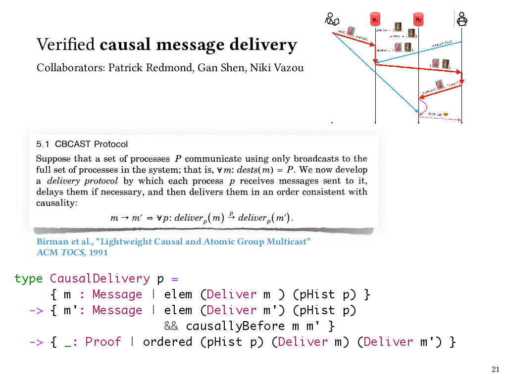
A classic protocol for ensuring causal message delivery in the case of broadcast messages is known as the CBCAST protocol, short for “causal broadcast”. This protocol was introduced by Ken Birman et al. in the early 90s in the context of their Isis system for fault-tolerant distributed computing.
The protocol ensures that when a process receives a message, that message is delayed if necessary and then delivered, meaning applied to that process’s state, only after any causally preceding messages have been delivered. In particular, if the send of message m happens before the send of message m’, in the sense of Lamport’s happens-before relation, then we know that on all processes, the delivery of m has to precede the delivery of m’. In CBCAST this is done by using vector clocks to represent causal dependencies, and delaying messages in a queue on the receiver’s side until it’s okay to deliver them. The deliverability check is done by comparing the receiving process’s vector clock with the vector clock of the message.
In our recent work, my students and I have implemented Birman et al.’s CBCAST protocol in Liquid Haskell, and we’ve used Liquid Haskell to verify that a causal delivery property holds of our implementation.
Here’s a simplified look at how we can use refinements in Liquid Haskell to express the type of a process that observes causal delivery. So, a process keeps track of the events that have occurred on it so far, including any messages it’s delivered – and that sequence of events comprises its process history. This type, CausalDelivery, says that if any two messages m and m’ both appear in a process history as having been delivered, and m causally precedes m’, then those deliveries have to appear in the process history in an order that’s consistent with their causal order. So this is essentially taking the definition of causal delivery from the paper and turning it into a property that we can enforce about a process.
Now that we’ve defined this type, the verification task is to ensure that for any process history that could actually be produced by a run of the CBCAST protocol, this causal delivery property holds.
Verifying a causal delivery protocol
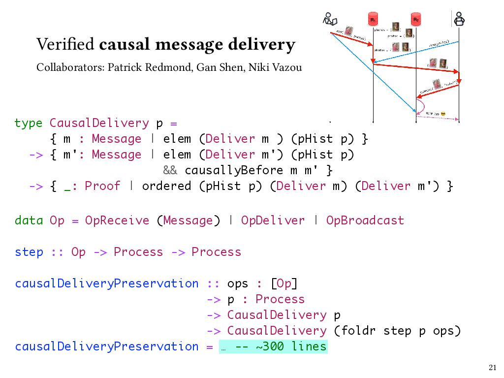
The way that we accomplish this is to express the CBCAST protocol in terms of a state transition system, where states represent the states of processes, and state transitions are the operations that broadcast, receive, or deliver messages. Here, the Op type represents those three kinds of state transitions, and the step function takes us from process state to process state.
We can then prove a property that I’ve called causalDeliveryPreservation here, which says that if a process observes causal delivery to begin with, then any process that could result from a sequence of state transitions produced by the protocol will observe causal delivery, too.
This took a few hundred lines of Liquid Haskell code to prove, with the most interesting part, of course, being the part that dealt with deliver operations.
I think there are a couple of interesting things to point out about this result. First of all, we found that the real key was implementing the protocol in terms of a state transition system. This wasn’t the way it was described in the original paper, although of course all the ideas were there. But we found that that’s what we needed to do to be able to express and prove properties like this, and it took a while for us to arrive at that design, even though it seems obvious in retrospect.
Second, I want to note that this protocol is entirely agnostic to the content of messages. It only looks at the causal metadata attached to messages, not the messages themselves. Now, there are downsides to this choice. If you’re implementing an end-to-end system, then you might be able to make smarter choices about message delivery if you know something about the semantics of the messages you’re dealing with. For instance, a message that might be deemed undeliverable by the causal broadcast protocol might be deliverable faster under your custom semantics. On the other hand, choosing to be agnostic to message contents means that we now have a general, verified causal message broadcast library that can sit at the foundation of many applications.
The hierarchy of needs
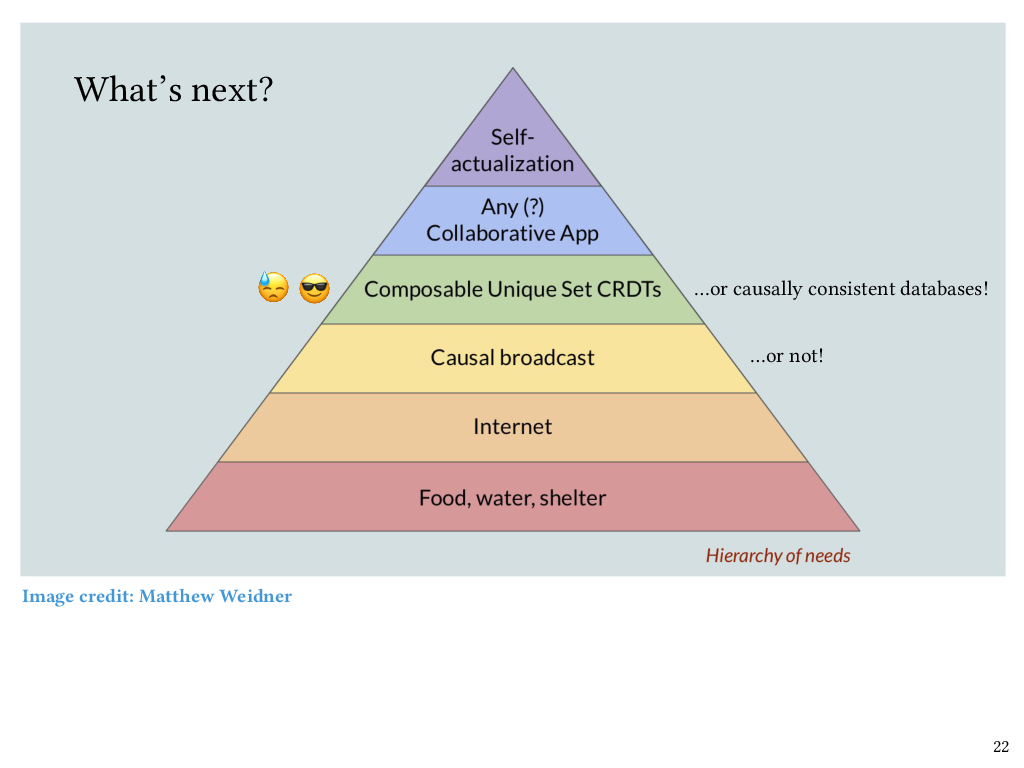
We’re now coming to the end of my talk, but if I’m going to talk about causal broadcast as being foundational, then I can’t help but show this delightful image, which I can’t take credit for – this image was created by Matt Weidner, who is currently a PhD student at CMU. The idea here is that once basic needs are covered – food, water, shelter, internet – then causal broadcast sits just above that, as a foundation for CRDTs and therefore collaborative software.
I mentioned earlier that some of our CRDTs took strenuous proof effort to verify, and part of the reason for that is because those CRDTs did not make an assumption of causal message delivery from the underlying network. However, now that we do have this new work on verified causal broadcast, my claim is that it will be easier to carry out those CRDT commutativity proofs, and I’d like to go back and revisit that work and build on top of causal broadcast. Conversely, some CRDTs don’t actually need causal broadcast to be strongly convergent, like, for instance, the counter CRDT I showed earlier, and in fact, my claim is that the ones that don’t need causal broadcast are exactly the ones that Liquid Haskell could verify the commutativity of automatically. For the ones that do need causal broadcast, the verification task, not to mention the implementation of the CRDTs themselves, ought to get simpler now that we have causal broadcast to build on top of.
I also want to add that CRDTs aren’t the only thing that can sit at this level of the hierarchy. Once you have causal broadcast it also becomes relatively straightforward to implement a causally consistent database. There’s already been a lot of nice work from the PL community on verification of the causal consistency, but as far as I’m aware, that work doesn’t factor out the causal broadcast protocol into its own separately verified layer, which is what we’ve done. So we think that it should be possible to verify causal consistency in a modular way on top of causal broadcast, and that’s one of the things we want to look at next.
Are we there yet?
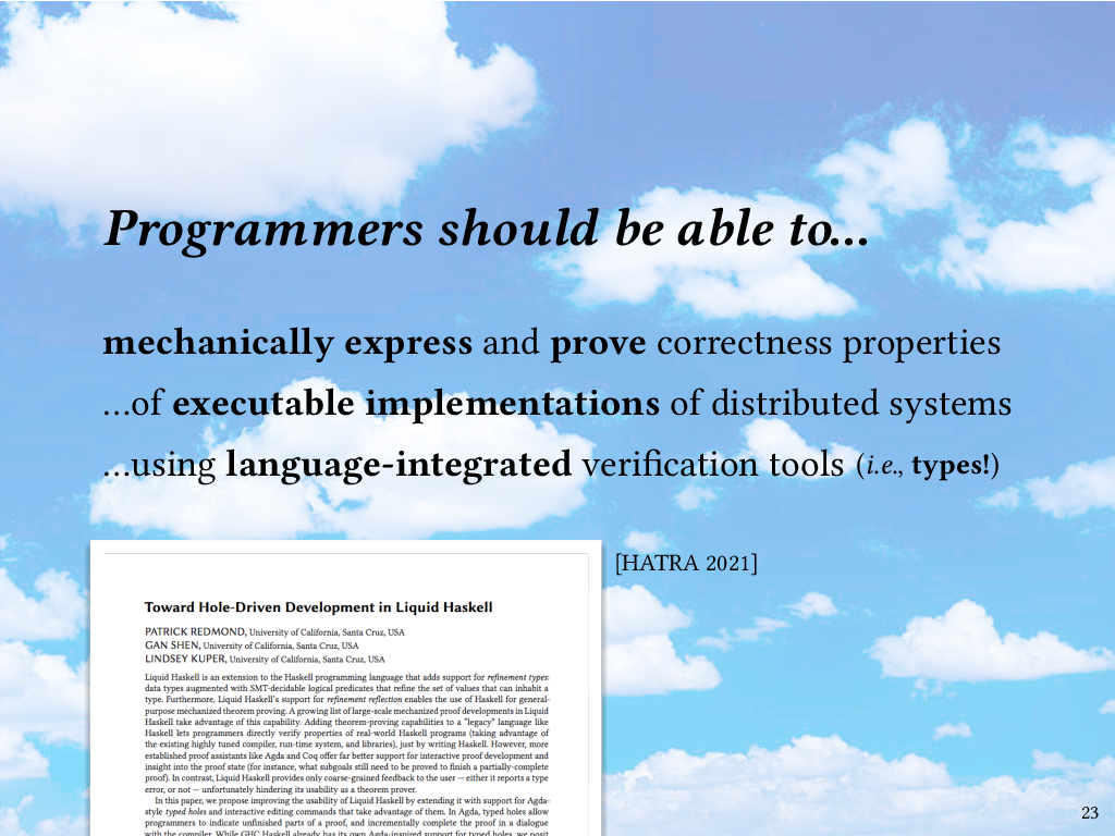
As I wrap up the talk, I want to come back to this blue-sky vision I mentioned earlier: that programmers should be able to mechanically express and prove rich correctness properties of executable implementations of distributed systems, using the same industrial-strength language that they use for the implementations themselves. Are we there yet? Our results so far suggest that with Liquid Haskell, it is possible. Unfortunately, I think it’s still way too hard to do.
Thanks to refinement reflection, Liquid Haskell can be used to turn Haskell into a proof assistant, and make no mistake, I think it’s great that this is possible at all. But developing long proofs in Liquid Haskell is quite painful. Part of the problem is that more established proof assistants like Agda and Coq offer far better support for interactive proof development and insight into the proof state (for instance, what subgoals still need to be proved to finish a partially-complete proof). In contrast, Liquid Haskell provides only very coarse-grained feedback – either it reports a type error, which means your proof isn’t done, or not, which mean it is. My students and collaborators and I have been thinking about how to improve the situation, and one of our proposals is to extend Liquid Haskell with support for Agda-style typed holes, and interactive editing commands that take advantage of them. Typed holes would allow programmers to indicate unfinished parts of a proof, and incrementally complete the proof in a dialogue with the compiler. While GHC Haskell already has its own Agda-inspired support for typed holes, but we think that typed holes would be especially powerful and useful if combined with Liquid Haskell’s refinement types and SMT automation. We published a short paper about this idea at the HATRA workshop last year, but there’s still a lot of work to do, so I would invite collaboration from anyone who’s interested in helping out here.
Conclusion
To conclude, we saw that we can use Liquid Haskell’s refinement types to express properties about the convergence of replicated data structures, and use Liquid Haskell’s refinement reflection and proof combinators to prove those properties extrinsically. Likewise, we can express and prove properties about the order in which broadcasted messages are delivered at a process, which should enable easier implementation and verification of applications on top of the messaging layer, whether it’s CRDTs or anything else. While Liquid Haskell is up to the task, we still think it could be a lot easier to use, and we look forward to continuing to improve it.
Thank you for listening!
-
As longtime readers of this blog might already know, my dirty secret about how I prepare for talks is that I often write them out word for word. What I write down may not exactly match what I actually say when I give the talk, but writing prose is how I organize the ideas in the first place. If the prose doesn’t hang together, it usually means that the ideas need more work. ↩
Comments