A few months ago, my group at Intel Labs began sponsoring and collaborating with a team of researchers at Stanford who are extending the capabilities of automated verification tools to formally verify properties of deep neural networks used in safety-critical systems. This is the second in a series of two posts about that work. In the previous post, we looked at what “verification” means, a particular system that we want to verify properties of, and what some of those properties are. In this post, we’ll dig into the verification process itself, as discussed in the Stanford team’s paper, “Reluplex: An Efficient SMT Solver for Verifying Deep Neural Networks”.
If you haven’t yet read the previous post, you may want to read it for background before continuing with this one.
Verification approach
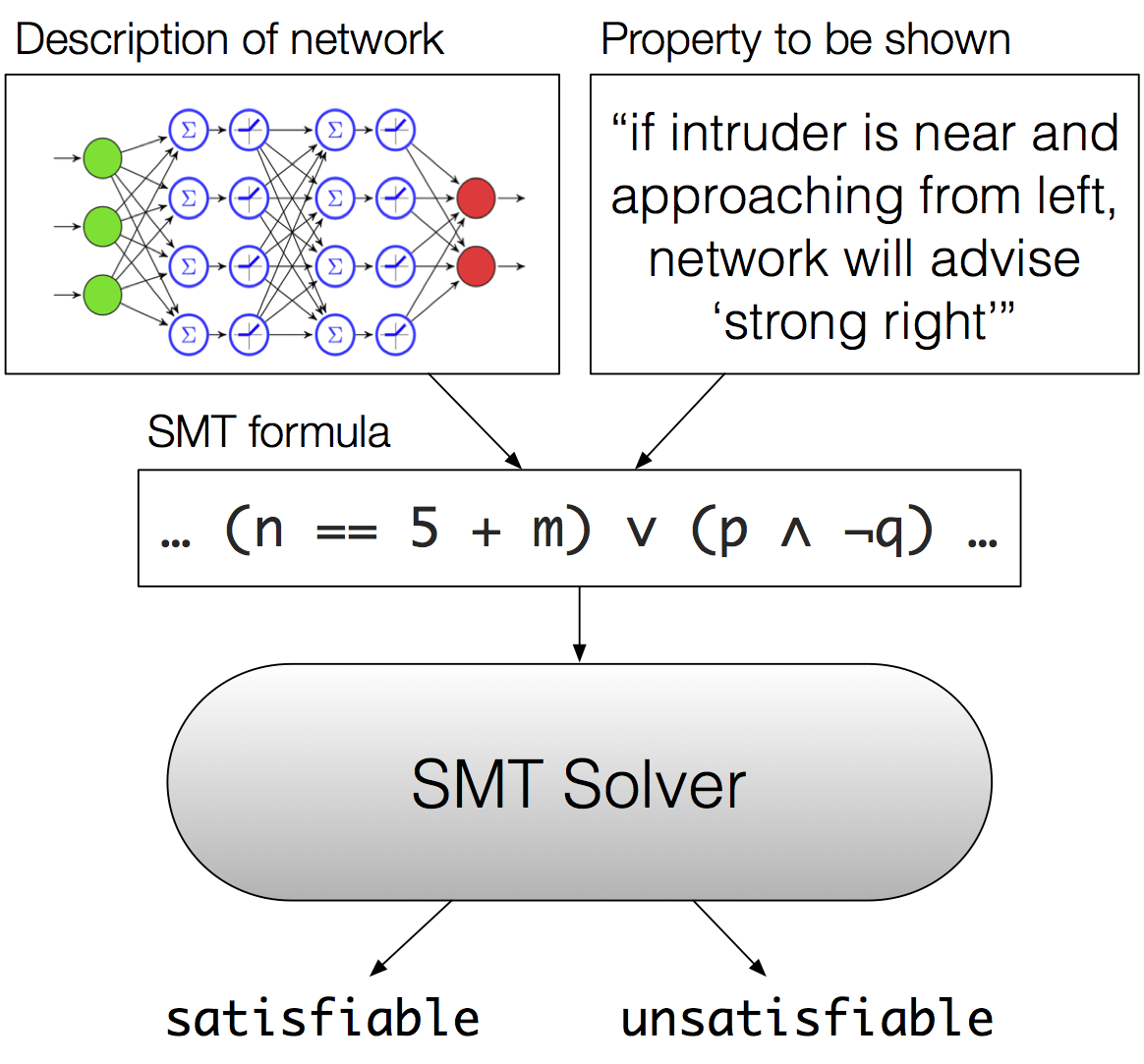
When we left off, we had described a neural network representation of the collision avoidance policy used by the ACAS Xu aircraft collision avoidance system. We had also discussed some properties that we’re interested in verifying about that network – for instance, the property that if an intruder aircraft is near and approaching from the left, the network will produce a “strong right” advisory. Let’s consider how we could use an SMT solver to show that such properties hold.
Our first step will be to take the trained network and encode it as a huge Boolean formula. Every unit in the network will become a variable in the formula, and everything that relates to each unit – weights, biases, and activations – is going to become part of the formula as well, as a constraint on that variable. We also encode the property we want to prove about the network as a part of our huge formula. Now we have something that we can determine the satisfiability (or unsatisfiability) of by feeding it to an SMT solver. But what does an SMT solver do, exactly?
An overview of our verification approach.
The
SAT problem
is the problem of determining whether a Boolean formula is
satisfiable. Given a formula containing only Boolean variables,
parentheses, and Boolean connectives (AND, OR, and NOT), the SAT
problem is to determine whether there is some assignment of “true” and
“false” to the variables that will make the formula true. This
problem is decidable,
meaning that it’s possible to write a computer program that can solve
it. (For instance, the
DPLL algorithm is a
well-known method for solving the SAT problem.) But it is famously
NP-complete, meaning
that there’s no known efficient solution to it.
SMT stands for satisfiability modulo theories, and the SMT problem is an extension of the SAT problem. The SMT problem is also about determining whether or not a formula is satisfiable, but in the case of SMT, the formula can be more complicated: instead of necessarily being just a Boolean formula, it can also contain other things – for instance, numbers. To determine the satisfiability of these fancier SMT formulas, we need to evaluate them according to the rules of what’s called a theory.
In our case, the particular theory we’re concerned with is the theory of linear real arithmetic. Linear real arithmetic formulas can contain equations or inequalities over the real numbers; the variables in them can be real numbers instead of just Booleans; and we can do addition, subtraction, and multiplication operations. In fact, when I wrote above that we were encoding our neural network and the property we wanted to prove about it as a Boolean formula, that was a lie – it’s actually a linear real arithmetic formula. The formula can also still have everything that a Boolean formula has (Boolean variables, parentheses, and Boolean connectives), so the whole thing might be something like a conjunction of equations over real numbers.
SAT problems are always decidable, but with SMT problems, the choice of the theory we’re working with determines whether or not the problem is decidable, and so we speak of decidable theories – those for which the SMT problem is decidable.1 Linear real arithmetic turns out, conveniently for us, to be a decidable theory.
Once we’ve handed our formula off to the SMT solver, we let the solver crank on the problem for many hours or days until it determines that the formula is either satisfiable or unsatisfiable. We’re working with a decidable theory, so in principle, the solver will eventually have an answer for us. In practice, though, SMT solving is often quite slow, and we may not have time to wait for the solver to finish. Much of SMT solving research therefore involves trying to find more efficient ways to determine the satisfiability of a formula.
The virtues of laziness
There are traditionally two approaches to implementing an SMT solver:
The eager approach is to take SMT formulas and essentially compile them down to a Boolean SAT formula that can be solved with an off-the-shelf SAT solver. As long as we’re dealing with a decidable theory, it’s possible to do this, in much the same way that we can compile code in a high-level language to machine code. However, when we compile to a plain old Boolean SAT formula, we lose the ability to apply domain knowledge from whatever theory we started with. For instance, we might like the solver to be able to exploit the fact that 3 plus 4 equals 4 plus 3 (or, in general, the fact that addition is commutative). The solver can do that easily if it’s working at a level of abstraction that makes it easy to express concepts such as equality and addition, but it’s harder to do if we only have Boolean formulas to work with.
<img src="https://decomposition.al/assets/images/lazy-smt-solver-architecture.png alt="The architecture of a lazy SMT solver." />The architecture of a lazy SMT solver.
The lazy approach combines an underlying SAT solver with various theory solvers that are each specific to a particular theory. This illustration (a modified version of one in a presentation by Clark Barrett) shows, at a high level, the architecture of a lazy SMT solver. The boxes at the top labeled “UF”, “Arithmetic”, and so on are various theory solvers. The theory solvers interact with the underlying SAT solver and gradually build up an answer to the question of whether a formula is satisfiable or not. In between, a solver core coordinates the two-way communication between the SAT solver and the theory solvers.
Although it was only pretty recently that I began learning about SMT solver internals, the notion of exploiting domain knowledge for efficiency reasons was immediately familiar to me. My lab’s work on ParallelAccelerator makes use of the idea that having a high-level representation of programmer intent enables domain-specific compiler optimizations that would be difficult or impossible otherwise. As I wrote recently, the promise of high-performance domain-specific languages is that they can offer efficiency not in spite of how high-level they are, but in fact because of how high-level they are. With lazy SMT solving, it’s a similar story: if we can do certain domain-specific optimizations at the level of the theory solver, then the satisfiability of a formula can be determined a lot more efficiently than if we eagerly compiled it to a Boolean formula right away. (And we really need all the help we can get in terms of efficiency, because, after all, we’re working with problems that are NP-complete!)
In the particular setting of verifying properties of deep neural networks, the ability to be lazy and handle things at the level of a theory solver turns out to be especially crucial. In our case, recall that we’re dealing with a network that uses ReLU activation functions. Those ReLU functions have to be represented somehow in the formula that we give to the solver. What our Stanford collaborators found is that dealing with ReLUs really must be done at the level of a theory solver instead of at the lower SAT-solver level, or the problem would be intractable. The key contribution of their Reluplex paper is a novel way to lazily handle ReLU activations. In some cases, treating ReLUs lazily can make the difference between a problem being solvable in a couple of days, and not being solvable in our lifetimes.
The lesson that I think we can take away from this is that if we want to be able to use SMT solver technology to verify things about neural networks, it’s not good enough just to express the networks and the properties we want to prove about them as formulas that we can pass to the solver. We need to build specialized theory solvers that are equipped for dealing with neural networks, and especially for dealing with activation functions. In fact, having looked at this problem for a few months now, I’ve come to believe that one reason why progress on neural network verification has been slow thus far is that most of the existing research has tried to use existing SMT solvers as black boxes. It’s tempting to use an existing solver in an off-the-shelf fashion, but I think that the reason why the Stanford team has had more success is that they’ve been willing to go under the hood, hack on solver internals, and develop a theory solver that’s well suited for dealing with ReLUs.
Lazily handling ReLU activations
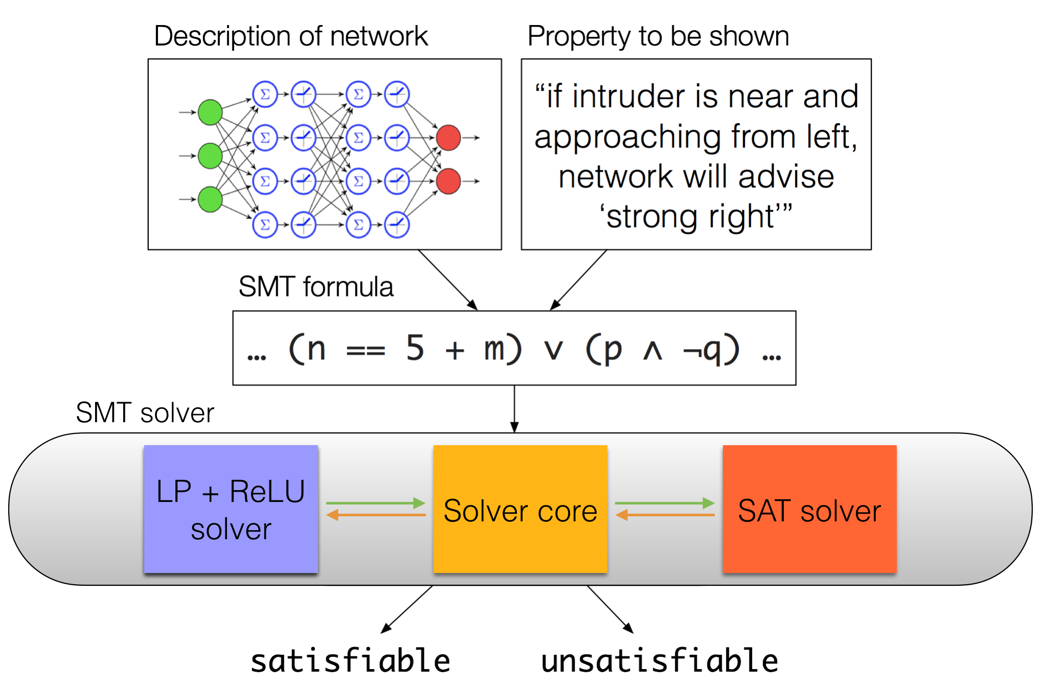
Now that we’ve talked a bit about SMT solver internals, we can return to our description of the high-level verification approach we’re taking and expand out the “SMT solver” part of the picture to be a bit more detailed.
An expanded overview of our verification approach.
We’ve discussed how, with lazy SMT solving, we can have different theory solvers tailored to particular theories, and that for our problem, we’re using what’s known as the theory of linear real arithmetic. A convenient thing about the theory of linear real arithmetic is that if our formula is written in a certain way – in particular, if it’s written as a conjunction of atomic linear-real-arithmetic formulas – then we can just use an off-the-shelf linear programming (LP) solver as our theory solver. That is to say, for certain kinds of linear real arithmetic formulas, LP solving coincides with SMT solving.
In our case, we’re almost able to take advantage of this happy coincidence. There’s just one catch: activation functions. Even ReLU activation functions, which are just about the simplest kind of activation function that a neural network can have, can’t be expressed as a conjunction of atomic formulas in our theory. Why? Recall that the ReLU activation function takes the maximum of its input and zero. So, it has to be expressed as a disjunction – either the input is less than zero and the output is zero, or the input is greater than zero and the output is the same as the input. This throws an annoying wrench in our ability to solve the problem with an LP solver.2 What’s more, disjunctions are especially troublesome for solver efficiency, because both disjuncts have to be checked.3 Since the result of each ReLU activation in a network can be either zero or nonzero, if the network has \(N\) ReLU activations, then there are \(2\^{N}\) disjuncts in the formula that we’re passing to the solver.
What the Stanford team found is that they could take an existing LP solver and extend it just enough to be able to handle ReLUs. Their prototype solver implementation, Reluplex, extends GLPK, an open-source LP solver. They do this by adding support for a new “ReLU” predicate that can appear in the formulas that we pass to the solver, which are otherwise just ordinary linear real arithmetic formulas.
Most of the time, these ReLU predicates can be dealt with lazily, meaning that the solver doesn’t have to split them into disjunctions. Instead, it can leave them unsplit and proceed with trying to solve the rest of the problem. Often, some other constraint in the problem will tell the solver whether a ReLU is going to be zero or nonzero, and so it can use that information to avoid exploring both disjuncts. It’s still not exactly fast to run the solver, but lazily handling ReLUs is enough to make many problems tractable that would be intractable otherwise.
What can we verify about the ACAS Xu DNN-based policy representation?
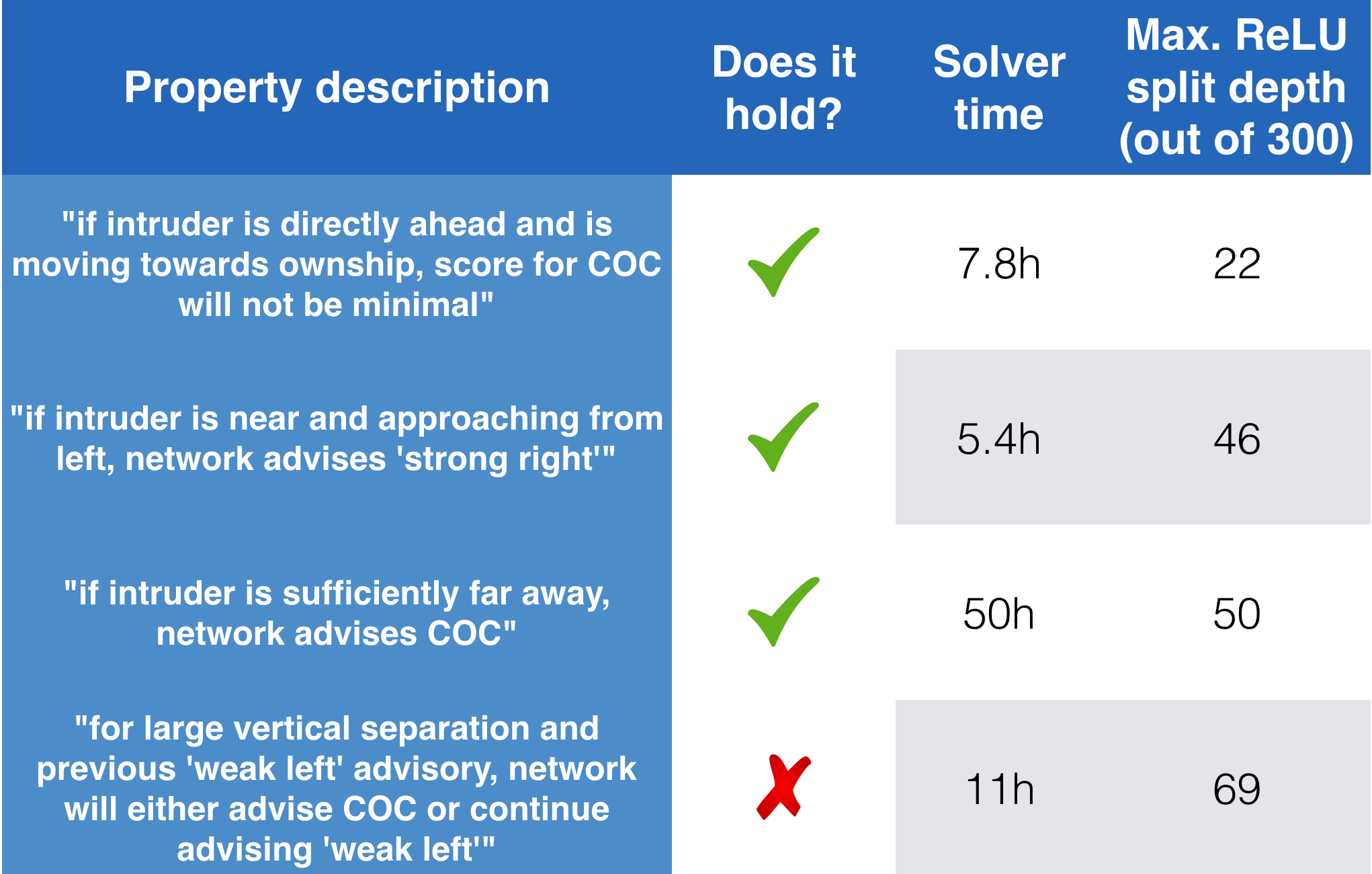
Using Reluplex, the Stanford team was able to prove (or disprove) a number of properties about the deep neural network that implements the ACAS Xu collision avoidance policy. In the below table, I’ve picked out four particular properties that I think are interesting; the full list of properties they showed is in their paper, along with many more details that I’m leaving out here.
Some properties of the ACAS Xu DNN that Reluplex was able to prove or disprove.
The first property says that if the intruder plane is directly ahead and is moving towards the ownship, the score for the clear-of-conflict advisory will not be minimal – in other words, the network will advise something other than clear-of-conflict. (In this setting, the lowest score is the best, so we want the score for at least one other advisory to be lower that the score for clear-of-conflict.) The solver showed that this property holds, and it took about 7.8 hours to verify.
The last column of the table bears a bit more discussion. First, we need to clarify one point about the network description that is passed to the solver. In the previous post, we saw that there are five discrete possibilities for the “previous advisory” (\(a\_{\mathit{prev}}\)) input to the network – COC, weak left, weak right, strong left, and strong right. Furthermore, for the “time until loss of vertical separation” (\(\tau\)) input, we consider only nine discrete possibilities: 0, 1, 5, 10, 20, 40, 60, 80, and 100 seconds. Because these two dimensions of the input space are discrete, it is possible to divide up the network into a family of 45 (= \(9 * 5\)) independent sub-networks that can be trained individually. Splitting up the network in this way means that we can dispatch to the appropriate sub-network and do inference on that sub-network instead of on the full-sized network, which is faster than doing inference on the full network. This was done for performance reasons, but it also has the happy side effect of making verification easier, since the solver can consider the sub-networks independently (potentially in parallel), and for some properties (say, if a property is vacuously true for all but one of the values of \(a\_{\mathit{prev}}\) or \(\tau\)), we may only need to consider one or a few of the sub-networks.
Even when only considering one sub-network, though, the solver has a lot of work to do. Each sub-network has 300 ReLU activations, meaning that there are \(2\^{300}\) possible combinations of zero or nonzero output for each ReLU. \(2\^{300}\) is a big number, and if it were necessary to explore both possibilities for each ReLU, then these properties would be intractable to verify in any reasonable amount of time. Thankfully, this is where the lazy ReLU technique described above comes in. For each of the properties we consider, the last column in the above table tells us what the maximum ReLU split depth was when the solver ran, averaged across all of the sub-networks under consideration. The split depth for the first property, for example, is 22, which tells us that the solver was able to avoid exploring both possibilities most of the time. \(2\^{22}\) isn’t tiny, but it’s a lot smaller than \(2\^{300}\)!
The second property in the table says that if the intruder is near and approaching from the left, the network will give a “strong right” advisory. The solver took about 5.4 hours to verify this property, and the maximum ReLU split depth of 46 shows that it was again able to avoid splitting ReLUs into disjuncts most of the time, although not as often as for the first property.
The third property I’ve listed is interesting: it says if the intruder is sufficiently far away, the network will advise that we’re clear of conflict. One might think that this property isn’t very important; after all, it wouldn’t be so bad to err on the side of caution and have a plane turn at a time when it was actually clear of conflict and didn’t really have to turn. However, issuing turn advisories when they aren’t really necessary is wasteful and, for piloted aircraft, can lead to alarm fatigue, so we do care about this property. In this case, it took about 50 hours for the solver to prove the property, reaching a maximum ReLU split depth of 50.
Finally, the fourth property I’ve listed here is one that the solver was actually able to disprove; that is, the solver was able to find a counterexample. It says that if the vertical separation between the planes is large and the previous advisory was ‘weak left’ (making this a case where we only need to consider one of the 45 sub-networks to exhaustively verify the property), then either the network will advise that we’re clear of conflict or it will continue advising ‘weak left’. The solver was able to find a particular input that violated the property. As the paper explains, “This confirmed the existence of a discrepancy that had also been seen in simulations, and which will be addressed by retraining the DNN.”
Verifying adversarial robustness
The Reluplex paper also considers the problem of verifying robustness of the ACAS Xu DNN to adversarial inputs. An adversarial input is a slight perturbation of an input that causes the network to misclassify it. Proving that a network is globally adversarially robust for a given size \(\delta\) of perturbation – that is, that the network will not misclassify any input that has been perturbed by at most \(\delta\) – still seems out of reach for networks the size of the ACAS Xu DNN. For now, what we can do is prove a local adversarial robustness property for a given \(\delta\) and a given input \(x\) – something that’s been explored in previous work on verifying neural networks with SMT solvers. The local adversarial robustness property for a given \(\delta\) and \(x\) says that perturbations to \(x\) of size at most \(\delta\) will not be misclassified by the network.
The Stanford team was able to use their prototype solver to prove (or disprove) local adversarial robustness for the ACAS Xu DNN for a few arbitrarily chosen combinations of \(\delta\) and \(x\).4 Proving or disproving these properties took anywhere from a few seconds to a few hours, depending on the \(x\) and \(\delta\) in question. Empirically, the results in the paper show that in general, the bigger the \(\delta\), the longer it takes to verify the property if it holds (which makes sense). On the other hand, in cases where local adversarial robustness does not hold, it never takes more than about twenty minutes to find a counterexample, and sometimes it’s much faster than that. (However, there are known fast techniques for finding adversarial inputs when they do exist, so the real purpose of using an SMT solver is to verify the absence of such inputs for a given \(x\) and \(\delta\).)
What’s next?
The solver that the Stanford team has developed so far is just a prototype, and it can’t yet handle everything that we want it to handle. For instance, one of its shortcomings is that it only handles networks that have ReLU activation functions. For the next version, which is already under development, we’re planning to support more kinds of activation functions; I have some ideas about how to do that. We also want to be able to handle more network architectures beyond the fully-connected networks that we support today. My hypothesis is that we can use a technique similar to what we use for ReLUs to handle the max pooling layers used in convolutional networks. And eventually, we’d like to explore more ways to speed up verification, whether that means parallelizing the solver, finding ways to simplify networks so that they’re more amenable to verification, or something else that we haven’t thought of yet.
Finally, we want to apply the tool to more networks, especially those used in safety-critical systems. If you think you have a network that we should be trying to verify properties of and that you think our solver (or the next version of it) should be able to handle, please get in touch!
Conclusion
In this post and the previous one, I’ve given an overview of our Stanford collaborators’ work on an SMT solver for verifying properties of safety-critical neural networks, and where I’d like to see the project go next. What are the high-level takeaways from what we’ve covered?
I suspect that deep learning in safety-critical systems is probably here to stay. Therefore, rather than insisting that DNNs are unverifiable, my view is that we should get to work on improving verification technology to handle how safety-critical software is now being built. From the Reluplex work, we’ve seen that it is possible to formally verify interesting properties of safety-critical DNNs using SMT solvers.
However, I think the most important takeaway from this work is that it’s not enough to just use off-the-shelf solvers as black boxes. We need to be willing to dig into solver internals. In particular, it seems to me that we need to invest in developing new theory solvers that are well suited for DNN problems and make use of laziness. We don’t necessarily need to start from scratch – we can leverage existing work, as Reluplex leverages existing LP solving technology – but we do need to be willing to build new theory solvers. Doing so could make the difference between only being able to handle toy-sized networks, and being able to scale to realistic problem sizes in reasonable amounts of time. There’s a lot more to do here, and we’re just getting started.
Thanks to Clark Barrett, Justin Gottschlich, Guy Katz, Mykel Kochenderfer, and Harold Treen for their feedback on drafts of this post.
Formally, a theory is a set of sentences (that is, logical formulas with no free variables in them) that are true according to some interpretation. When the problem of determining membership in that set is decidable, we say that the theory is a decidable theory. I find “(un)decidable theory” – and “(un)decidable set”, for that matter – to be harder to understand than the equivalent “theory/set for which the problem of determining membership is (un)decidable”, because I like to think of problems as the things that are fundamentally decidable or undecidable. That said, this is kind of a silly hangup I have, because the whole notion of a “problem” is ultimately defined in terms of sets anyway! ↩
Disjunction can be encoded using a combination of conjunction and negation, but the result wouldn’t be a conjunction of linear-real-arithmetic atoms, which is what we would need to be able to use an unmodified LP solver for this problem. ↩
Why do we need to check both disjuncts of a disjunction? We’re trying to show a safety property, meaning that we want to show that a (usually bad) thing can’t happen. The way to show such a property with an SMT solver is to provide the solver with a formula saying the opposite – that the bad thing can happen – and then try to show that that formula is unsatisfiable. If you have a formula with a lot of disjuncts, you have to then go through and check each disjunct, in case it’s the one that could lead to the bad thing happening. (If we were merely trying to show an existence property, then we could stop checking disjuncts as soon as we found one that satisfied the property.) What this means for our purposes is that the number of disjuncts in a formula makes a big difference to solver running time. ↩
I ran some of the adversarial experiments myself with Reluplex and got results similar to those in the paper. I also picked out a few other inputs to try (dis)proving adversarial robustness for and was able to do so. You can try it yourself, too – the code has particular inputs hard-coded, but it’s easy to change. ↩

Comments