
The optimization that wasn’t
Between mid-2015 and mid-2017, I spent a lot of time on performance measurement for the ParallelAccelerator package for Julia. I curated a collection of workloads of interest and tried to automate the process of benchmarking them as much as I could. Many of the workloads had originally been written in Matlab or Octave, and the Julia versions had been ported from those.
One such workload – now available as an example program that comes with the ParallelAccelerator package – was an implementation of the two-dimensional wave equation, ported from an Octave implementation with the permission of the original author. The wave equation models the vibrations of a wave across a surface, such as a drum head when struck or the surface of a pond when hit by a drop of water. Using the wave equation, you can derive a formula that will tell you where each point on that surface will be on the next time step, based on that point’s position in the current and previous time steps.
Here’s an animated GIF of the simulation running, created using Winston.jl and ImageMagick:
This animation shows us looking down at our simulated surface from above. The circles emanating outward from the center are waves created by the “drop of water” that’s just hit the surface. (There’s also something else coming from the left; that’s the “dynamic source” described in the original author’s article.)
The most interesting part of the code is the part that implements the wave equation, which we sped up using ParallelAccelerator’s runStencil construct, as described in section 3.3 of our paper. But this post isn’t about that – it’s about a mistake we made when porting the original Octave code to Julia!
What was current is now past; what was future is now current
Leaving aside ParallelAccelerator and runStencil, let’s take a look at the Julia code that was directly ported from Octave. The code uses three two-dimensional arrays, called p, c, and f for “past”, “current”, and “future” respectively, to keep track of the positions of points on the surface. Each iteration of the main loop of the simulation uses the wave equation to compute a new version of f, based on the contents of p and c.
The part of the code we’re concerned with comes at the end of the main loop. After computing the new f, the simulation moves one step into the future. It updates the contents of p to those of c, then updates the contents of c to those of f – and around we go to beginning of the loop to compute the next f using the wave equation again. The code that does the end-of-loop updates to p and c looks like this (where s is the size of the array along each dimension):
p[1:s, 1:s] = c[1:s, 1:s]
c[1:s, 1:s] = f[1:s, 1:s]
These two lines of Julia code are identical to the Octave code they were ported from, except that Octave uses parentheses for array indexing instead of square brackets.
Oops!
One of my colleagues proposed that instead of having all those nasty array indices, we ought to be able to just write
p = c
c = f
to update the two arrays at the end of the loop. Not only did the change make the code more concise, it was also faster when we benchmarked it. We reasoned that the new version of the code was faster because, instead of copying the contents of c into p and the contents of f into c every time through the loop, the p = c; c = f version merely moved pointers around.
Some months later, late in 2015, I happened to run the code with plotting turned on. We usually never ran with plotting, because we wanted to benchmark only the time it took to compute the arrays, not the time it took to visualize the results of that computation.1 With plotting enabled, I expected to see something like the above animation, but I was surprised by what I saw instead. After a couple of frames, the animation seemed to just…stop.
Based on that symptom, I bet some of you have already correctly diagnosed the bug, but I didn’t yet understand what was going on. At first, I thought that something was wrong with the plotting code, but I looked and didn’t see any problems there. Then I remembered the change we’d made several months previously, and I decided to change the two lines that updated p and c back to the old version that used explicit indices, just to see what would happen.
When I made that change, the visualization showed the simulation running like it should, no longer seeming to stop after a couple of steps. I didn’t know why switching back to the old version of the code had fixed the problem, but I checked in the change with a TODO for myself to “figure out what’s going on with the array assignment bug”.
The next day, I went back to figure out what was going on and busted out everyone’s favorite debugging tool: good ol’ box-and-pointer diagrams.
Copying arrays: correct, but inefficient
Let’s say that we’ve just computed f on our first time through the loop. Suppose p points at turquoise, c points at orange, and f points at purple:
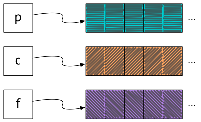
It’s now time to update p and c to prepare for our next trip through the loop, where we’ll compute the next value of f. Let’s first consider the more verbose version of the code that uses explicit array indexing. In this version of the code, we update p and c by copying the contents of c into p, and then the contents of f into c:
The contents of the array originally pointed to by c have been copied over into the array pointed to by p, and the contents of the array originally pointed to by f have been copied over into the array pointed to by c. So now p points at orange, and c points at purple.
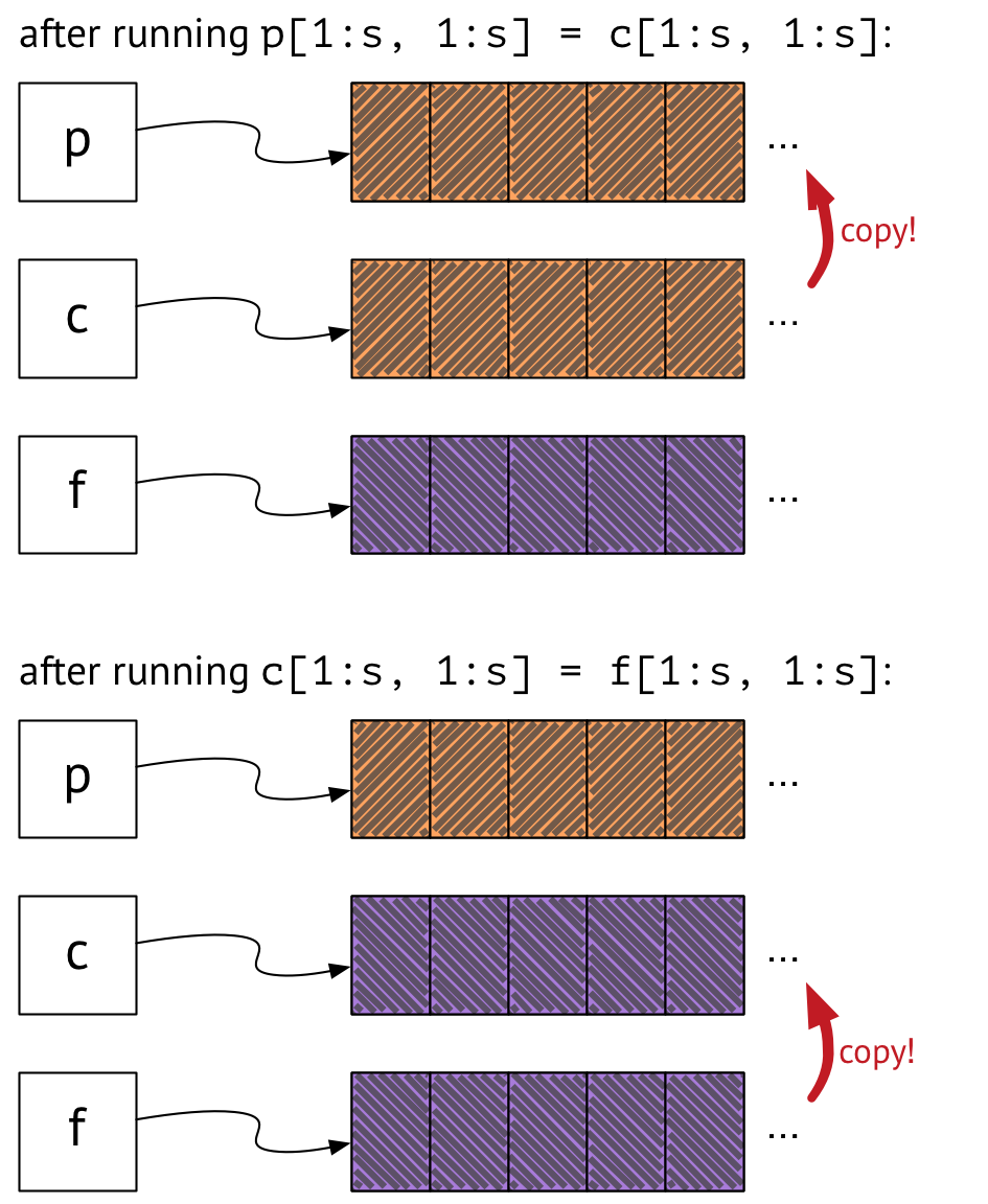
f also points at purple, but not for long: on the next trip around the loop, we compute the new contents of f – let’s say they’re pink. Then we update p and c again, as before:
Now p, c, and f point to purple, pink, and pink, respectively, and we’re ready for our next trip around the loop to re-compute f again.
Moving pointers around: efficient, but…
The above approach works, but it involves a lot of copying. Wouldn’t it be nice if we could simply swap pointers around instead of having to copy the contents of arrays? That’s what the p = c; c = f version of the code was supposed to do. Let’s see what happens when we run it.
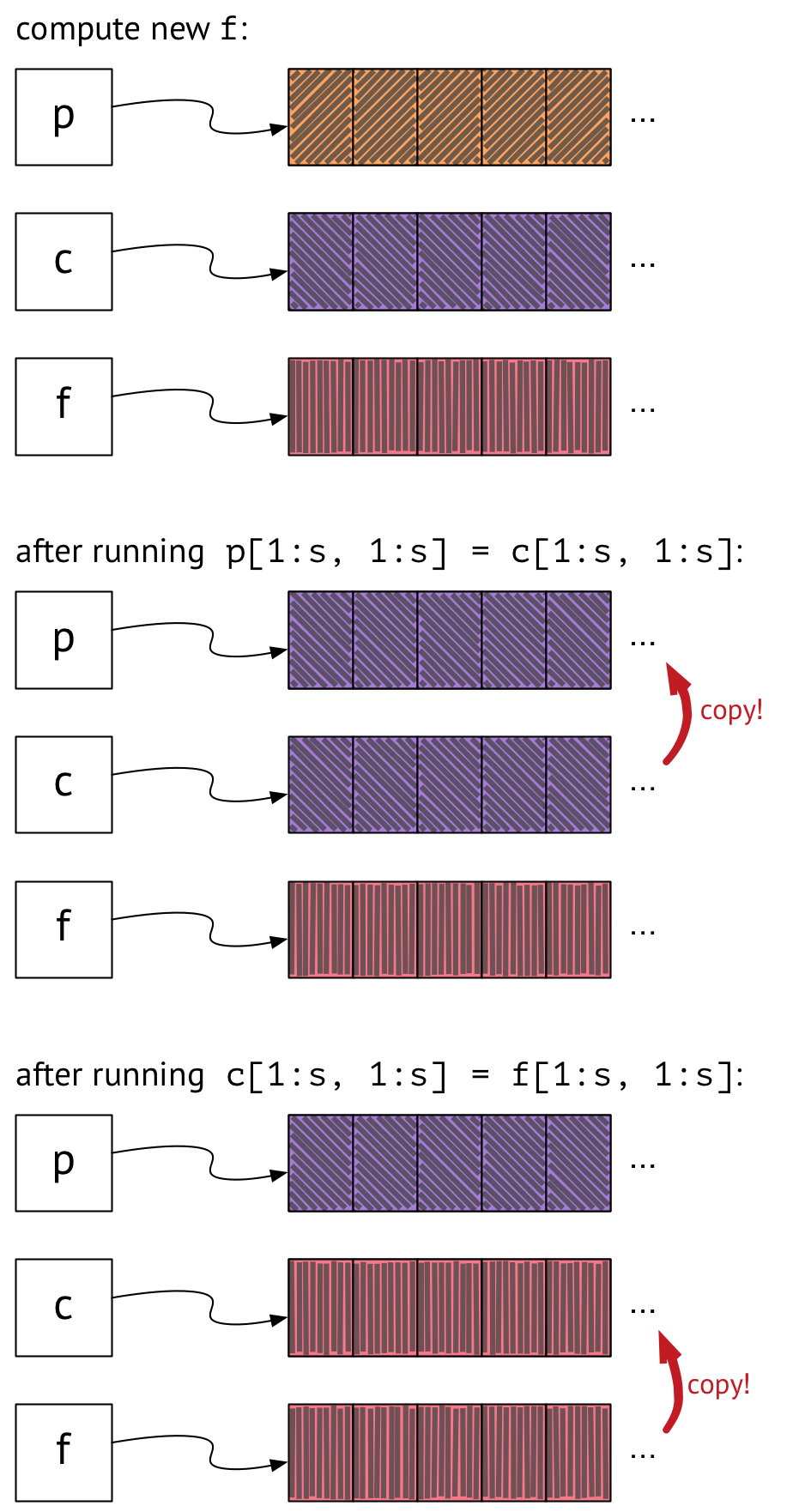
Once again, here’s our starting state after computing f on our first time through the loop:
Next, we update p to point to where c is pointing, and we update c to point to where f is pointing:
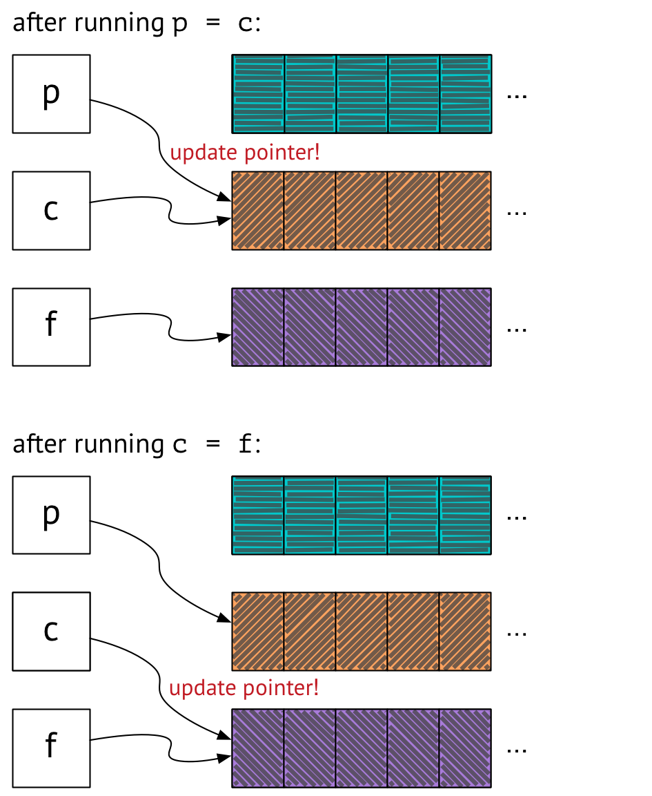
Now we’ve got p pointing at orange, and c and f both pointing at purple. This state seems to be Observably Equivalent™ to the state we were in before, when we were copying arrays around – and we accomplished it by just moving a couple of pointers! Hooray!
But wait – what happens on the next trip through the loop?
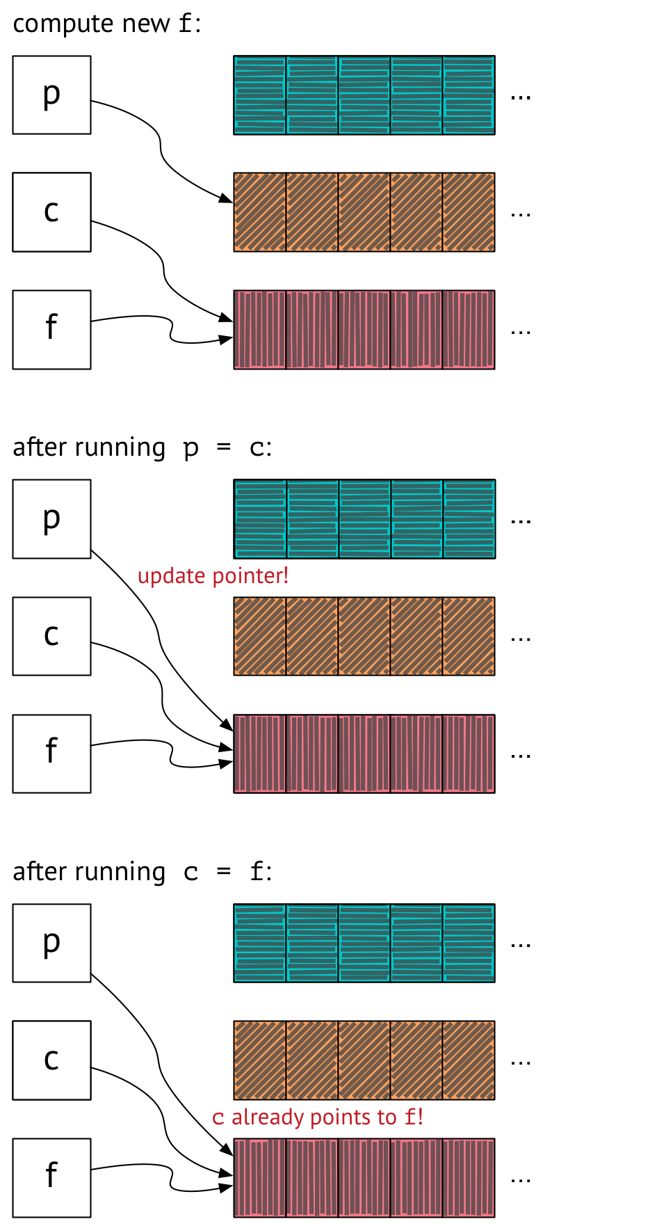
We compute the new contents of f, which are pink, as before. But now when we run p = c, we update p to point to what c is pointing to – and that’s f! And running c = f is a no-op, since c already points to what f is pointing to. So now all three of p, c, and f are pointing at the same array. Now that this is the case, all future assignments of p = c and c = f will also be no-ops, and our code won’t work.
Moving pointers around, correctly
Thankfully, there’s an easy solution to this problem that still lets us avoid copying arrays around every time we go through the loop. Instead of writing
p = c
c = f
we can introduce a temporary variable, like so:
tmp = p
p = c
c = f
f = tmp
When we do this, here’s what things look like at the end of the first time step:
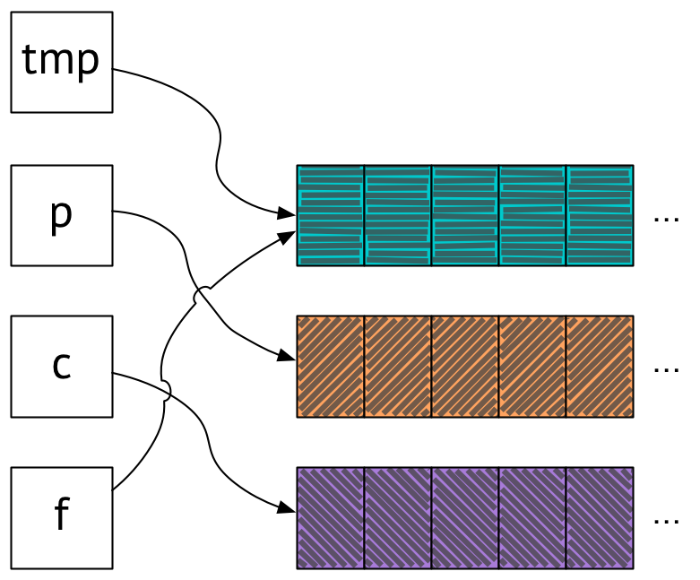
As in the other versions we’ve seen, p points at orange and c points at purple. We have f pointing at turquoise, but the contents of the array f points to aren’t important, since they’re about to change on the next time through the loop. The important thing is that neither p nor c point to where f points, so updating the contents of f will not affect the contents of p or c, which is how we got into trouble last time.
At the end of the next time step, all our pointers rotate:
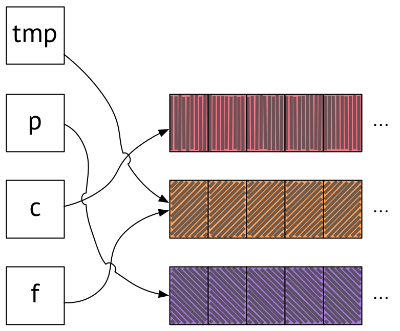
Now p points to purple and c points to pink, which is what we want, and again, neither one points to the same place as f, and the simulation continues to run correctly for the remaining time steps. Note that our orange and purple arrays are in the same place they were before – they didn’t have to move! Only the variables pointing to them changed.
I got rid of the array-copying code and replaced it with the pointer-swapping version that uses tmp. Now, not only did our code not do any unnecessary copying, but it had the added bonus of being correct!
Questions to ponder
The issue here turned out to be an example of a classic pointer-aliasing bug: we had two variables pointing to the same place when they shouldn’t have been. But why did the bug manifest in the way it did, by making the animation appear to stop after the second frame? It seems clear that the behavior of the code was going to be wrong in some way as a result of the aliasing bug, but why was it wrong in that particular way?
Here’s something that might be a clue: after fixing the pointer-aliasing bug, if we replace the occurrence of p in the wave equation with c, then we also get the behavior where the animation appears to freeze after the second frame – even though f[x, y] doesn’t, in general, work out to be the same thing as c[x, y] for a given x and y. Why?
Finally, would it have worked to just write f = p; p = c; c = f instead of introducing tmp? I’ll leave that one as an exercise for the reader, too.
A note about Julia versus Octave
In the Julia docs, the “noteworthy differences from MATLAB” section mentions the fact that Julia arrays are assigned by reference: “After A=B, changing elements of B will modify A as well.” That didn’t happen with p[1:s, 1:s] = c[1:s, 1:s]; c[1:s, 1:s] = f[1:s, 1:s], because expressions like c[1:s, 1:s] are what are known as array “slice” expressions, and slices always make copies of the data being referred to.
In Matlab (and Octave), arrays are not assigned by reference, and modifying the original won’t modify the copy. So it presumably would have been fine to write p = c; c = f in Octave, instead of the version with slices. (In fact, I don’t know why the original Octave code wasn’t just p = c; c = f – perhaps someone reading this can enlighten me.) As it is, the code was “accidentally correct” when first ported to Julia, because it happened to be written using slices that referred to the entire array.
In general, though, slices can address just some portion of an array – that’s the point of slices! In Julia, if you want to refer to a part of an array but you don’t want the copying overhead that comes with using slices, you can use a new feature called views; Spencer Russell has a nice blog post about that.
Thanks to Cameron Finucane, Veit Heller, and Valentin Churavy for giving feedback on drafts of this post or discussing aspects of it with me.
-
In fact, the majority of the running time of the simulation went to plotting the results of the computation rather than to the computation itself, but ParallelAccelerator couldn’t do anything to speed up plotting, so we just turned off plotting and only benchmarked the part of the code that we could speed up. This, of course, was cheating. For instance, the plain Julia version of the computation ran in about 4 seconds, whereas the ParallelAccelerator version ran in about 0.3 seconds, and so we reported an order-of-magnitude speedup. But plotting took something like 20 seconds for each version, so if we’d had plotting enabled, the ParallelAccelerator version would have run in 20.3 seconds compared to 24 seconds for the plain Julia code – a measly 15% speedup. ↩
Comments