The case of the missing frames

In my last post, I wrote about a wave equation simulation that I spent a lot of time with as part of my ParallelAccelerator for Julia benchmarking effort. To illustrate the post, I made an animated GIF of the simulation running:

This animation shows a simulated surface of a pond seen from directly above. We can see circles emanating from the center of the plot, representing waves spreading out from the point where a drop of water has hit the pond. But something's wrong -- the animation seems jerky, like frames are being dropped. Why?

Over the course of the simulation, we can see circles emanating from the center of the plot, similar to how waves spread out in circles from the point where a drop of water hits a still pond. There are also waves coming from somewhere off to the left that interact with the waves coming from the center.

The simulation runs for 5000 time steps and then loops back to the beginning. There should be a frame of animation for each tenth time step, plus one initial frame – 501 frames in all. But something’s wrong – the animation looks choppy in places, as though some of the frames are missing. What gives?

I first noticed this frame-dropping behavior a long time ago, the first time I ran the code with visualization turned on. Because I was watching the visualization “live” as the code ran, though, I figured that my computer was just dropping frames because it was slow or busy with some other task. I thought the frames were there, just not being shown. It wasn’t until I made the above GIF and watched it that I suspected that something was wrong, because the GIF also looked like it was missing frames, even though it wasn’t running “live”. Hmmm.

I went back to look at the Julia code that did the plotting:

if mod(t/dt, 10) == 0
    plot = Winston.imagesc(c)
    Winston.display(plot)
end

This code uses the Winston.jl 2D plotting package to plot an image for each tenth time step using the imagesc function, then displays that image on the screen. To make the above GIF, I’d also added an additional line of code that would save each image out to a file using Winston’s savefig function, with sequentially numbered file names:

if mod(t/dt, 10) == 0
    plot = Winston.imagesc(c)
    Winston.display(plot)
    Winston.savefig("figure" * @sprintf("%03d",t*1000) * ".png")
end

Since there’s a frame for every tenth time step, if we were on time step number 8, this code would save the image as figure008.png, for instance.

Then I stitched together all the PNG files into an animation with a shell command using good ol’ convert:¹

convert -delay 10 -loop 0 *.png wave-animation.gif

The shell globbing conveniently takes care of putting the images in the correct order as frames in our GIF: figure000.png, representing the initial state of the simulation, would be followed by figure001.png and then figure002.png, all the way up to figure500.png. All this seemed to be working correctly; the frames weren’t being assembled in the wrong order. I still didn’t understand what was causing the jerkiness in the animation. But then I checked how many frames I actually had:

$ ls -1 *.png | wc -l
389

389? That was a lot fewer than the 501 I was supposed to have! I went back and looked at the plotting code again:

if mod(t/dt, 10) == 0
    plot = Winston.imagesc(c)
    Winston.display(plot)
    Winston.savefig("figure" * @sprintf("%03d",t*1000) * ".png")
end

And then, finally, the problem jumped out at me. The line if mod(t/dt, 10) == 0 is supposed to make sure that we only plot every tenth time step of the simulation. t represents the amount of time that has passed since the beginning of the simulation, and dt represents the amount of time that goes by with each time step. In my code, as in the original Octave code from which it was ported, dt is set to 0.0001. Having dt be a variable means that we can easily change the time resolution of the simulation by making dt larger or smaller.

Why are we checking if mod(t/dt, 10) is equal to zero? As the author of the original code explains: “t/dt will return a natural number which represents the number of timesteps since the simulation has started. The modulo of this number and 10 will return the remainder of the division of these two numbers. Consequently comparing the modulo with 0 will only return true every tenth time the count variable t was incremented […].”

The problem here is that, at least after porting to Julia from Octave, t/dt can’t be counted on to return a natural number! Take, for instance, the third time step. At this time step, t is 0.0003, and so t/dt ought to be 0.0003 divided by 0.0001, which is 3. But because of floating-point inexactness, t/dt comes out to something like 2.9999999999999996, and therefore mod(t/dt, 10) also comes out to 2.9999999999999996.

The first dropped frame seems to occur on the 90th time step, when t reaches 0.009. Then, t/dt comes out to 89.99999999999999 instead of 90, and so mod(t/dt, 10) comes out to 9.999999999999986 instead of 0. From that point on, frames are dropped here and there, whenever t/dt works out to be something that isn’t an integer on a time step that happens to be a multiple of 10.

I tried logging the values of t, t/dt, and mod(t/dt, 10) at each time step as the code ran. There were some stretches of time where t/dt always came out integral:

...
t = 0.2104, t/dt = 2104.0, mod(t/dt, 10) = 4.0
t = 0.2105, t/dt = 2105.0, mod(t/dt, 10) = 5.0
t = 0.2106, t/dt = 2106.0, mod(t/dt, 10) = 6.0
t = 0.2107, t/dt = 2107.0, mod(t/dt, 10) = 7.0
t = 0.2108, t/dt = 2108.0, mod(t/dt, 10) = 8.0
t = 0.2109, t/dt = 2109.0, mod(t/dt, 10) = 9.0
t = 0.211, t/dt = 2110.0, mod(t/dt, 10) = 0.0
t = 0.2111, t/dt = 2111.0, mod(t/dt, 10) = 1.0
t = 0.2112, t/dt = 2112.0, mod(t/dt, 10) = 2.0
t = 0.2113, t/dt = 2113.0, mod(t/dt, 10) = 3.0
t = 0.2114, t/dt = 2114.0, mod(t/dt, 10) = 4.0
t = 0.2115, t/dt = 2115.0, mod(t/dt, 10) = 5.0
t = 0.2116, t/dt = 2116.0, mod(t/dt, 10) = 6.0
t = 0.2117, t/dt = 2117.0, mod(t/dt, 10) = 7.0
t = 0.2118, t/dt = 2118.0, mod(t/dt, 10) = 8.0
t = 0.2119, t/dt = 2119.0, mod(t/dt, 10) = 9.0
t = 0.212, t/dt = 2120.0, mod(t/dt, 10) = 0.0
t = 0.2121, t/dt = 2121.0, mod(t/dt, 10) = 1.0
t = 0.2122, t/dt = 2122.0, mod(t/dt, 10) = 2.0
t = 0.2123, t/dt = 2123.0, mod(t/dt, 10) = 3.0
t = 0.2124, t/dt = 2124.0, mod(t/dt, 10) = 4.0
t = 0.2125, t/dt = 2125.0, mod(t/dt, 10) = 5.0
...

But during other stretches of time, t/dt would be non-integral as often as not:

...
t = 0.0483, t/dt = 483.0, mod(t/dt, 10) =3.0
t = 0.0484, t/dt = 483.99999999999994, mod(t/dt, 10) = 3.999999999999943
t = 0.0485, t/dt = 485.0, mod(t/dt, 10) = 5.0
t = 0.0486, t/dt = 485.99999999999994, mod(t/dt, 10) = 5.999999999999943
t = 0.0487, t/dt = 487.0, mod(t/dt, 10) = 7.0
t = 0.0488, t/dt = 488.0, mod(t/dt, 10) = 8.0
t = 0.0489, t/dt = 488.99999999999994, mod(t/dt, 10) = 8.999999999999943
t = 0.049, t/dt = 490.0, mod(t/dt, 10) = 0.0
t = 0.0491, t/dt = 490.99999999999994, mod(t/dt, 10) = 0.9999999999999432
t = 0.0492, t/dt = 492.0, mod(t/dt, 10) = 2.0
t = 0.0493, t/dt = 492.99999999999994, mod(t/dt, 10) = 2.999999999999943
t = 0.0494, t/dt = 493.99999999999994, mod(t/dt, 10) = 3.999999999999943
t = 0.0495, t/dt = 495.0, mod(t/dt, 10) = 5.0
t = 0.0496, t/dt = 495.99999999999994, mod(t/dt, 10) = 5.999999999999943
t = 0.0497, t/dt = 497.0, mod(t/dt, 10) = 7.0
t = 0.0498, t/dt = 497.99999999999994, mod(t/dt, 10) = 7.999999999999943
t = 0.0499, t/dt = 499.0, mod(t/dt, 10) = 9.0
t = 0.05, t/dt = 500.0, mod(t/dt, 10) = 0.0
t = 0.0501, t/dt = 500.99999999999994, mod(t/dt, 10) = 0.9999999999999432
t = 0.0502, t/dt = 502.0, mod(t/dt, 10) = 2.0
t = 0.0503, t/dt = 502.99999999999994, mod(t/dt, 10) = 2.999999999999943
t = 0.0504, t/dt = 504.0, mod(t/dt, 10) = 4.0
t = 0.0505, t/dt = 505.0, mod(t/dt, 10) = 5.0
t = 0.0506, t/dt = 505.99999999999994, mod(t/dt, 10) = 5.999999999999943
t = 0.0507, t/dt = 507.0, mod(t/dt, 10) = 7.0
t = 0.0508, t/dt = 507.99999999999994, mod(t/dt, 10) = 7.999999999999943
t = 0.0509, t/dt = 509.0, mod(t/dt, 10) = 9.0
t = 0.051, t/dt = 509.99999999999994, mod(t/dt, 10) = 9.999999999999943
t = 0.0511, t/dt = 510.99999999999994, mod(t/dt, 10) = 0.9999999999999432
...

Most interestingly of all, sometimes a pattern would emerge for a while – like here, for instance:

...
t = 0.2508, t/dt = 2508.0, mod(t/dt, 10) = 8.0
t = 0.2509, t/dt = 2509.0, mod(t/dt, 10) = 9.0
t = 0.251, t/dt = 2510.0, mod(t/dt, 10) = 0.0
t = 0.2511, t/dt = 2511.0, mod(t/dt, 10) = 1.0
t = 0.2512, t/dt = 2511.9999999999995, mod(t/dt, 10) = 1.9999999999995453
t = 0.2513, t/dt = 2513.0, mod(t/dt, 10) = 3.0
t = 0.2514, t/dt = 2514.0, mod(t/dt, 10) = 4.0
t = 0.2515, t/dt = 2515.0, mod(t/dt, 10) = 5.0
t = 0.2516, t/dt = 2516.0, mod(t/dt, 10) = 6.0
t = 0.2517, t/dt = 2516.9999999999995, mod(t/dt, 10) = 6.999999999999545
t = 0.2518, t/dt = 2518.0, mod(t/dt, 10) = 8.0
t = 0.2519, t/dt = 2519.0, mod(t/dt, 10) = 9.0
t = 0.252, t/dt = 2520.0, mod(t/dt, 10) = 0.0
t = 0.2521, t/dt = 2521.0, mod(t/dt, 10) = 1.0
t = 0.2522, t/dt = 2521.9999999999995, mod(t/dt, 10) = 1.9999999999995453
t = 0.2523, t/dt = 2523.0, mod(t/dt, 10) = 3.0
t = 0.2524, t/dt = 2524.0, mod(t/dt, 10) = 4.0
t = 0.2525, t/dt = 2525.0, mod(t/dt, 10) = 5.0
t = 0.2526, t/dt = 2526.0, mod(t/dt, 10) = 6.0
t = 0.2527, t/dt = 2526.9999999999995, mod(t/dt, 10) = 6.999999999999545
t = 0.2528, t/dt = 2528.0, mod(t/dt, 10) = 8.0
t = 0.2529, t/dt = 2529.0, mod(t/dt, 10) = 9.0
t = 0.253, t/dt = 2530.0, mod(t/dt, 10) = 0.0
t = 0.2531, t/dt = 2531.0, mod(t/dt, 10) = 1.0
t = 0.2532, t/dt = 2531.9999999999995, mod(t/dt, 10) = 1.9999999999995453
...

And again, later on:

...
t = 0.4943, t/dt = 4943.0, mod(t/dt, 10) = 3.0
t = 0.4944, t/dt = 4944.0, mod(t/dt, 10) = 4.0
t = 0.4945, t/dt = 4945.0, mod(t/dt, 10) = 5.0
t = 0.4946, t/dt = 4946.0, mod(t/dt, 10) = 6.0
t = 0.4947, t/dt = 4946.999999999999, mod(t/dt, 10) = 6.9999999999990905
t = 0.4948, t/dt = 4948.0, mod(t/dt, 10) = 8.0
t = 0.4949, t/dt = 4949.0, mod(t/dt, 10) = 9.0
t = 0.495, t/dt = 4950.0, mod(t/dt, 10) = 0.0
t = 0.4951, t/dt = 4951.0, mod(t/dt, 10) = 1.0
t = 0.4952, t/dt = 4951.999999999999, mod(t/dt, 10) = 1.9999999999990905
t = 0.4953, t/dt = 4953.0, mod(t/dt, 10) = 3.0
t = 0.4954, t/dt = 4954.0, mod(t/dt, 10) = 4.0
t = 0.4955, t/dt = 4955.0, mod(t/dt, 10) = 5.0
t = 0.4956, t/dt = 4956.0, mod(t/dt, 10) = 6.0
t = 0.4957, t/dt = 4956.999999999999, mod(t/dt, 10) = 6.9999999999990905
t = 0.4958, t/dt = 4958.0, mod(t/dt, 10) = 8.0
t = 0.4959, t/dt = 4959.0, mod(t/dt, 10) = 9.0
t = 0.496, t/dt = 4960.0, mod(t/dt, 10) = 0.0
t = 0.4961, t/dt = 4961.0, mod(t/dt, 10) = 1.0
t = 0.4962, t/dt = 4961.999999999999, mod(t/dt, 10) = 1.9999999999990905
t = 0.4963, t/dt = 4963.0, mod(t/dt, 10) = 3.0
t = 0.4964, t/dt = 4964.0, mod(t/dt, 10) = 4.0
t = 0.4965, t/dt = 4965.0, mod(t/dt, 10) = 5.0
t = 0.4966, t/dt = 4966.0, mod(t/dt, 10) = 6.0
t = 0.4967, t/dt = 4966.999999999999, mod(t/dt, 10) = 6.9999999999990905
t = 0.4968, t/dt = 4968.0, mod(t/dt, 10) = 8.0
t = 0.4969, t/dt = 4969.0, mod(t/dt, 10) = 9.0
t = 0.497, t/dt = 4970.0, mod(t/dt, 10) = 0.0
t = 0.4971, t/dt = 4971.0, mod(t/dt, 10) = 1.0
t = 0.4972, t/dt = 4971.999999999999, mod(t/dt, 10) = 1.9999999999990905
...

During these stretches, we get an inexact answer for every fifth value of t, whenever t has a 2 or a 7 in its fourth decimal place, and not for any other value of t. Other patterns show up elsewhere. Perhaps there’s something to be learned from studying these patterns. If you want to analyze the whole log of them, please be my guest!

Anyway, as is probably clear by now, we can fix the dropped-frames bug by rounding t/dt up to the nearest integer:

if mod(ceil(t/dt), 10) == 0
    plot = Winston.imagesc(c)
    Winston.display(plot)
    Winston.savefig("figure" * @sprintf("%03d",t*1000) * ".png")
end

With this fix, we have the correct number of frames:

$ ls -1 *.png | wc -l
501

And our convert command produces a lovely, smooth animation:

Here's that animation again, but now it's nice and smooth.

Ah! That’s better!

I updated my previous post to use the smooth animation instead of the choppy one. For comparison, here are the old and new versions, side by side. Since the smooth version has more than a hundred more frames than the choppy version, we can see that it also takes a bit longer to run:

Ugh, nasty! Ah, that's better.

Is there a lesson to be learned from all this? If the lesson of the previous post was that visualizing what your code is doing can be a helpful way to find bugs, perhaps the lesson here is to trust what the visualization shows you. In this case, our animation came out choppy for a reason. The other lesson here, I suppose, is to watch out for inexact fractions. In this case, d/dt was already in the code we were porting from, but that’s no excuse!

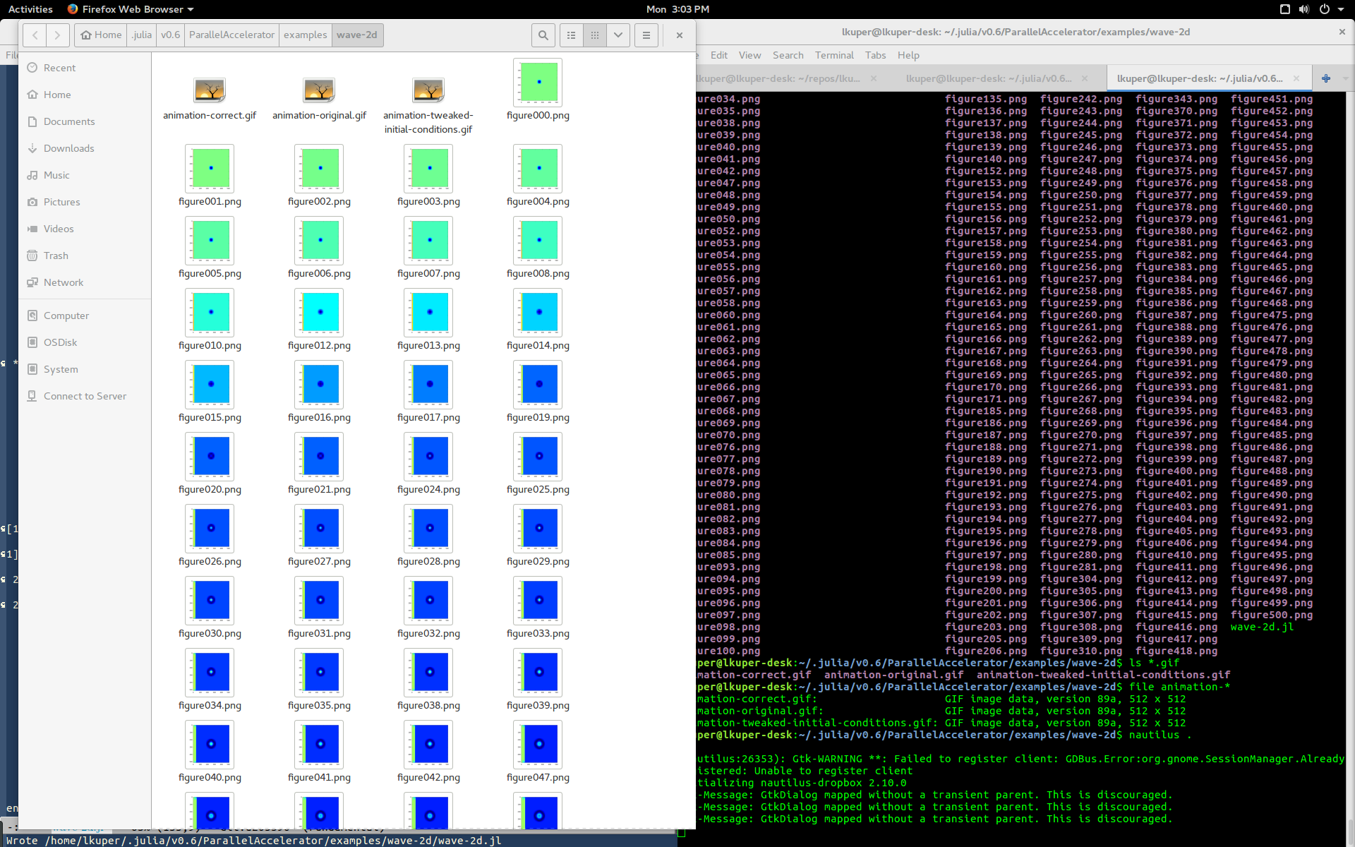
To conclude, here’s a process screenshot for Katherine Ye. I like the gradient thing going on here.

Note the missing frames.

Thanks to Cameron Finucane for a conversation that inspired this post.

1. Here’s something else that tripped me up at this stage: so, convert has a -loop option. I assumed that -loop 1 meant “loop” and -loop 0 meant “don’t loop”. But, no, in fact, the argument to -loop is the number of times you want your GIF to loop – except in the special case of 0, which means “loop infinitely”. So -loop 1 and -loop 0 had exactly the opposite of the behavior I expected! Oops. ↩