An example run of a matrix-based causal unicast protocol

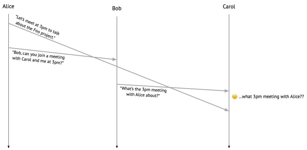
Suppose Alice messages Carol, saying “Let’s meet at 3pm to talk about the Foo project.” It then occurs to Alice that Bob should join the meeting, too, so she messages Bob, asking, “Can you join a meeting with Carol and me at 3pm?” Both messages go into the ether.

Bob sees the message from Alice and sends one to Carol: “What’s the 3pm meeting with Alice about?” But at this point, Carol hasn’t heard anything from Alice about a meeting yet, so she’s confused. Um…what 3pm meeting?

If you’ve ever found yourself in a situation like Carol’s, then you may have been the victim of an infamous distributed systems bug: a violation of causal message delivery!

A violation of causal message delivery. You may be entitled to compensation.

To understand what went wrong here, let’s consider the relationships between each of the messages that were sent. Alice sent a message to Carol before she sent one to Bob, so her message to Carol can be said to have happened before her message to Bob, in the sense of Lamport’s happens-before relation. In the same sense, Alice’s message to Bob can be said to have happened before Bob’s message to Carol, because Bob received Alice’s message before sending one to Carol. Because the happens-before relation is transitive, we can put those two relationships together to see that Alice’s message to Carol happened before Bob’s message to Carol – but that’s not the order that Carol saw them in! No wonder Carol is confused.

We can fix this problem by running a protocol that ensures causal message delivery: if a message \(m\) happens before a message \(m'\), then any process delivering both messages should deliver \(m\) before delivering \(m'\). “Delivery” here refers to something that happens to a message on the receiving end. A process has no control over the order in which it receives messages, but it can control when to do something (or not!) with each received message. Imagine a little mail clerk hanging out on each process, accepting incoming messages and choosing to either hand them off to the intended recipient (such as, say, Carol’s messaging app) – in other words, deliver them – or, perhaps, let them sit in the mail room for a while.

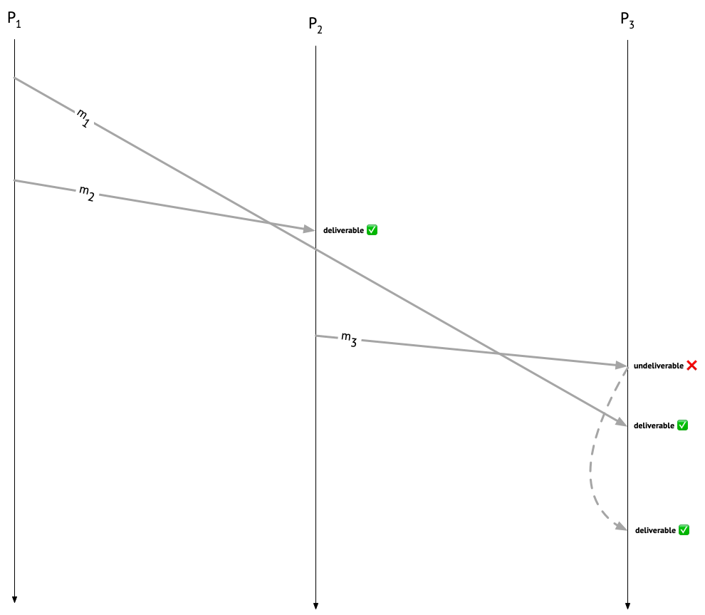
Let’s look again at our execution, giving Alice, Bob, and Carol the creative names \(P_1\), \(P_2\), and \(P_3\), respectively. We’ll call Alice’s message to Carol \(m_1\), Alice’s message to Bob \(m_2\), and Bob’s message to Carol \(m_3\). \(m_1\) causally precedes \(m_2\), and \(m_2\) causally precedes \(m_3\), so \(m_1\) causally precedes \(m_3\), and \(P_3\) should hold off on delivering \(m_3\) until it’s delivered \(m_1\). On the other hand, \(m_1\) and \(m_2\) can be immediately delivered at their respective recipients.

For this execution to observe causal delivery, P_3 should wait to deliver m_3 until after it's delivered m_1, even though it happened to receive m_3 first. The dashed arrow represents what our notional mail clerk on P_3 will do with m_3.

In this post, I’ll discuss a classic protocol for causal message delivery, published by Raynal, Schiper, and Toueg in 1991. It’s not the only way to ensure causal delivery of messages – for example, you could also do it by delaying messages on the sender’s side, rather than on the recipient’s side! – but that’s a story for another time.

Causal unicast is harder than causal broadcast

Interestingly, if we restrict things to the case where all the messages we want to send are broadcast messages – that is, if all messages are addressed to all recipients – then ensuring causal message delivery gets easier! I discuss how to implement causal broadcast in this lecture from my undergrad distributed systems class.

Unfortunately for Alice, Bob, and Carol, though, their messages are point-to-point, or unicast, messages, rather than broadcast messages. A causal broadcast protocol works under the assumption that every message will eventually arrive at every recipient. For example, under a causal broadcast protocol, upon receiving \(m_2\), \(P_2\) would queue it up and wait for \(m_1\) come along, since \(m_1\) causally precedes \(m_2\). If \(m_1\) were a broadcast message, that would indeed be the behavior we want – but in our scenario, \(P_2\) would be waiting forever for \(m_1\) to arrive!¹ So a causal broadcast protocol really won’t do, and our mail clerk needs a more nuanced way to determine whether a message is deliverable, taking into account not only causal precedence of messages, but also their intended destinations.

The causal broadcast protocol I teach my undergrads is more or less Birman et al.’s CBCAST protocol (which my group has spent a lot of time thinking about lately – check out our draft paper on mechanically verifying it!), which uses vector clocks to represent causal relationships between messages. In the CBCAST protocol, the vector clock attached to a given message tells you which messages causally precede that message, and who sent them. For the protocol I’ll discuss in this post, we’ll use a slightly more sophisticated clock data struture that also captures the extra information about message destinations that our mail clerk needs. You don’t have to understand vector-clock-based causal broadcast to understand this post, but it might make a good stepping stone, since it’s a simpler protocol.

Getting started

Let’s jump right in with implementing the causal unicast protocol! Each process will need to maintain two local data structures:

• A data structure for tracking how many messages (it thinks) each process has sent (and, importantly, to whom they’ve been sent).
• A data structure for tracking how many messages it has delivered from each process.

Following Raynal et al., at each process \(P_i\) we’ll use the names \(\mathit{SENT}_i\) and \(\mathit{DELIV}_i\) for these respective data structures.

For the \(\mathit{SENT}\) data structure, we can track sent messages in a two-dimensional, \(n \times n\) matrix², where \(n\) is the number of processes in the system, rows represent senders, and columns represent receivers. For example, the matrix

[ 0, 0, 1,
  2, 0, 0,
  0, 0, 0 ]

represents a state in which \(P_1\) has sent one message to \(P_3\) (that’s the 1 in the first row and third column), \(P_2\) has sent two messages to \(P_1\) (that’s the 2 in the second row and first column), and \(P_3\) hasn’t sent any messages yet. In general, an entry at index \(i,j\) tells you the number of messages sent by \(P_i\) to \(P_j\).

For the \(\mathit{DELIV}\) data structure, all we need is a vector. For example, the vector [0, 2, 1] represents a state in which a given process has delivered zero messages from \(P_1\), two messages from \(P_2\), and one message from \(P_3\).

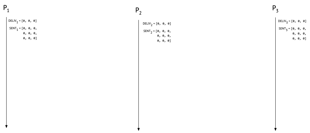
At the start of a run, nobody’s sent or delivered any messages, so both our matrix and our vector are going to be filled up with zeroes:

Ready to start running the causal unicast protocol.

Before we go on, an important caveat: we are assuming (as Raynal et al. do) that sent messages are eventually received at their destination. Without this assumption, our protocol would still be safe (i.e., processes would never deliver messages out of causal order), but it might not be live (i.e., messages could languish undelivered indefinitely). We are also assuming that we have a fixed set of participating processses. There are ways to deal with a dynamically changing set of participants, but they’re out of scope for this post. Finally, causal message delivery is (to paraphrase Sam Tobin-Hochstadt) an important but specific property; it’s not “message delivery system goodness”. There are myriad ways in which Alice, Bob, and Carol can still confuse each other even if they’re running this protocol, especially if they’re allowed to lie or otherwise behave maliciously.

With those disclaimers out of the way, we’re now ready to start sending (and hopefully delivering) messages!

Sending messages

In Raynal et al.’s protocol, whenever a process \(P_i\) sends a message to process \(P_j\), it should:

• Attach the current \(\mathit{SENT}_i\) to the message as metadata.
• Increment \(\mathit{SENT}_{i}[i, j]\) immediately after sending the message.

The metadata that \(P_i\) attaches to an outgoing message is a summary of the causal history of that message – it will tell the recipient what messages causally precede the current one.

Let’s see how this looks for \(P_1\) in our example run.

P_1 has sent two messages and updated its local state accordingly.

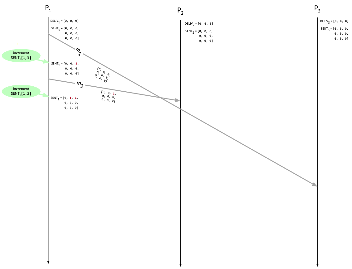
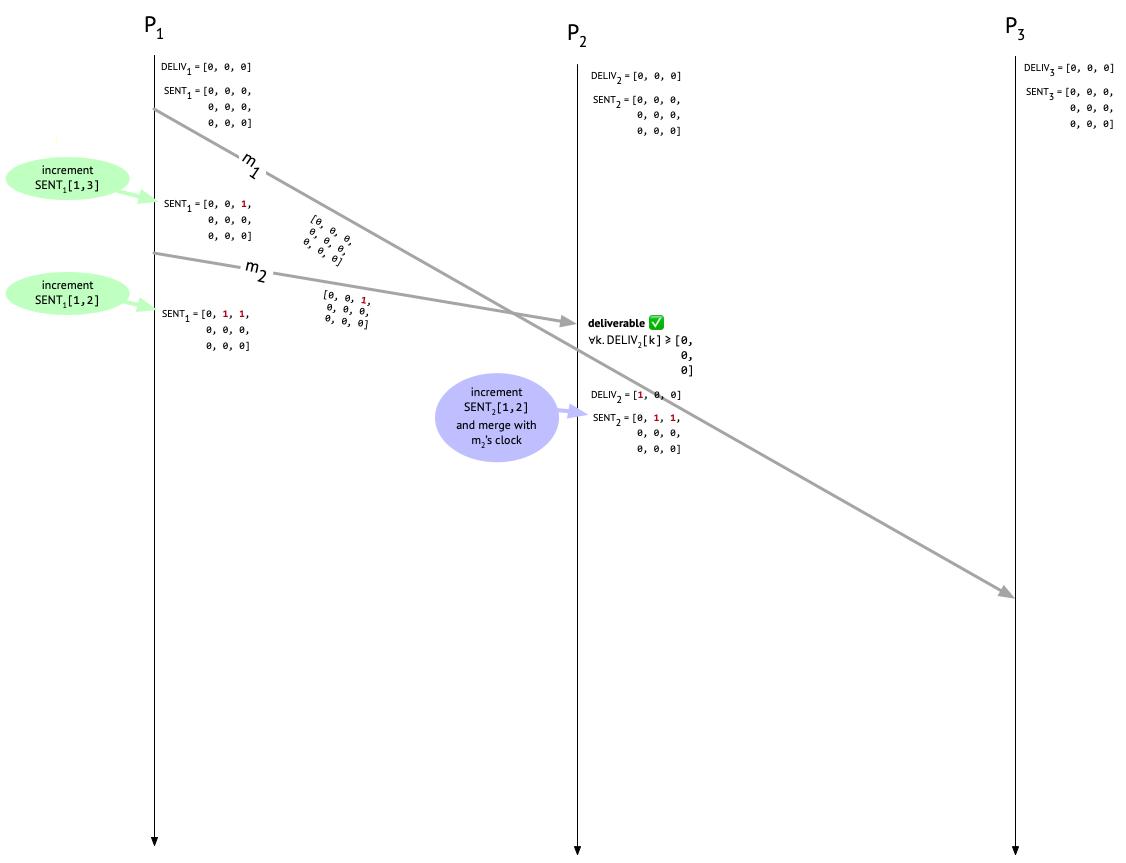
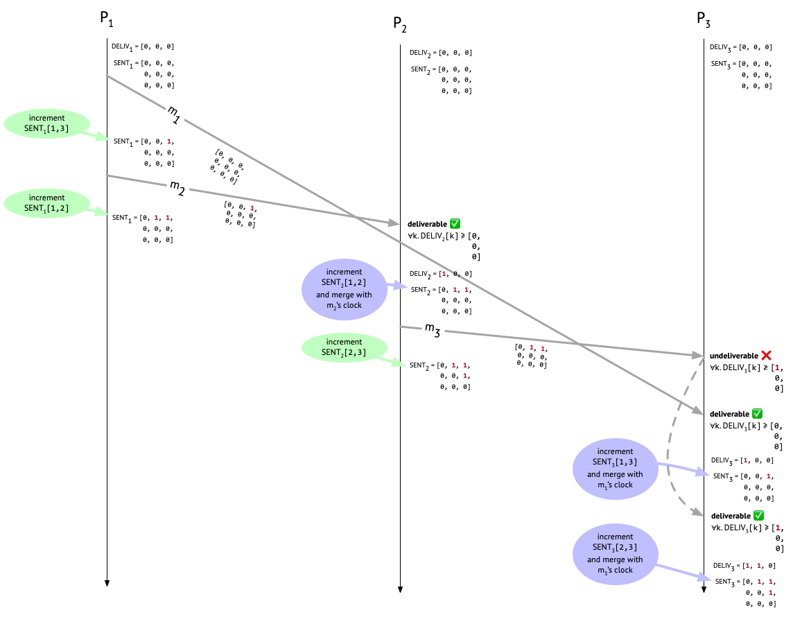
First, \(P_1\) sends \(m_1\) to \(P_3\) – this is Alice’s “Let’s meet at 3pm” message to Carol – and increments the appropriate entry in \(\mathit{SENT}_1\) to indicate that one message has been sent to \(P_3\). The attached metadata on \(m_1\) is from before the increment happened, so it’s all zeroes. Next, \(P_1\) sends \(m_2\) to \(P_2\) – this is Alice’s “Can you join the meeting at 3pm?” message to Bob – again attaching the current \(\mathit{SENT}_1\) (which now reflects the earlier send to \(P_3\)), and then incrementing the appropriate entry after the send. \(P_1\) hasn’t delivered any messages, so \(\mathit{DELIV}_1\) remains untouched.

So far, so good. Next, let’s look at what happens when these messages get to their intended recipients!

Delivering messages (or not)

Sooner or later, \(m_2\) will show up at \(P_2\). What should \(P_2\) do to determine whether the message is deliverable? Well, it needs to make sure that before delivering \(m_2\), it’s first delivered any causally preceding messages that are destined for it. \(P_2\) hasn’t delivered any messages at all yet when \(m_2\) shows up, as we can see from \(\mathit{DELIV}_2\).

To see whether it can deliver \(m_2\), \(P_2\) inspects the causal history metadata attached to \(m_2\). In fact, one message – \(m_1\) – did causally precede \(m_2\), and we can see that from the single non-zero entry in \(m_2\)’s metadata, which is in row 1 and column 3 because it was a message from \(P_1\) to \(P_3\). But does \(P_2\) care about that for the purposes of deciding whether to deliver \(m_2\)? No! For now, \(P_2\) only cares about the entries that are in its own column – column 2 – because those are the the messages that are actually destined for it. Since column 2 consists entirely of zeroes, \(P_2\) knows that there aren’t any messages out there that it needs to wait around for before delivering \(m_2\).

In general, the deliverability condition that a process \(P_i\) needs to check before delivering a message, say \(m\), from \(P_j\) is: For all \(k\), is \(\mathit{DELIV}_{i}[k] \geq \mathit{SENT}_{m}[k, i]\) (where \(\mathit{SENT}_{m}\) is the causal metadata attached to \(m\))?

The \(i\) index picks out the column of \(\mathit{SENT}_{m}\) that is relevant to \(P_i\)’s decision, since \(P_i\) only cares about messages destined for it. The \(k\) row index iterates over senders. The deliverability condition ensures that \(P_i\)’s already delivered messages (tracked in \(\mathit{DELIV}_{i}\)) are at least as up to date as \(P_j\)’s knowledge of the messages sent to \(P_i\) before \(m\). If that isn’t the case, then \(P_i\) had better not deliver \(m\) yet, because more messages that ought to be delivered before \(m\) are still on the way!

Since only column \(i\) of \(\mathit{SENT}_{m}\) figures into \(P_i\)’s deliverability check, why did \(P_j\) have to send the whole thing over, rather than just the \(i\) column? To answer this question, let’s look at what happens after a process delivers a message.

After delivering a message

Whenever a process \(P_i\) delivers a message \(m\) from \(P_j\), it needs to do three (!) things to maintain its local state:

• Increment \(\mathit{DELIV}_{i}[j]\), to record the newly delivered message \(m\).
• Increment \(\mathit{SENT}_{i}[j, i]\), to record the fact that \(m\) was sent by \(P_j\). We have to do this because \(P_j\) incremented its own \(\mathit{SENT}\) matrix after sending \(m\), rather than before. Otherwise, this step could just be folded into the next step.
• Update every entry in \(\mathit{SENT}_i\) to the maximum of itself and the corresponding entry in \(\mathit{SENT}_{m}\), the causal metadata attached to \(m\).

It’s that last step that’s the reason why \(P_j\) needed to send its entire \(\mathit{SENT}\) matrix over with \(m\): \(P_i\) needs the information about \(m\)’s entire causal history – not only the messages that also happen to be destined for \(P_i\) – because that information needs to be passed along in the causal metadata for any future messages that \(P_i\) might send.

Let’s look at how this plays out in our example run. \(P_2\) has decided that \(m_2\) is deliverable, and delivers it. \(P_2\) then carries out the three post-delivery steps. First, it updates \(\mathit{DELIV}_{i}\) from [0, 0, 0] to [1, 0, 0], to record that a message from \(P_1\) has now been delivered locally. Next, it increments \(\mathit{SENT}_2[1, 2]\) to record that \(P_1\) has sent a message to \(P_2\). \(\mathit{SENT}_2\) now looks like:

[0, 1, 0,
 0, 0, 0,
 0, 0, 0]

Finally, the last step: \(P_2\) merges the \(\mathit{SENT}_1\) metadata that came along with \(m_2\) into its own \(\mathit{SENT}_2\). Since \(\mathit{SENT}_1\) was

[0, 0, 1,
 0, 0, 0,
 0, 0, 0]

the result of this merge will be

[0, 1, 1,
 0, 0, 0,
 0, 0, 0]

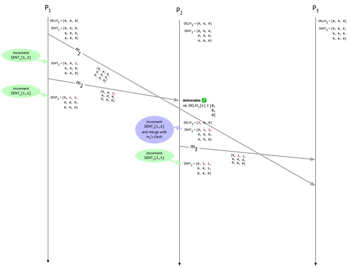
which should now agree with what \(P_1\) has for \(\mathit{SENT}_1\), since both \(P_1\) and \(P_2\) did an increment on their own side. Whew. Here’s what things look like now:

P_2 has delivered a message and updated its local state accordingly.

Bob’s fateful message to Carol

At this point, Bob has heard from Alice and is wondering what the 3pm meeting is about, so he messages Carol. This is message \(m_3\) in our example, and Bob attaches \(\mathit{SENT}_2\) to the message and increments the \(\mathit{SENT}_2[2,3]\) entry after doing the send. Now things look like this:

P_2 has sent a message, with causal metadata attached, and updated its local state accordingly.

We’ve reached the moment of truth: is the protocol going to prevent Carol from seeing Bob’s confusing message before seing Alice’s?

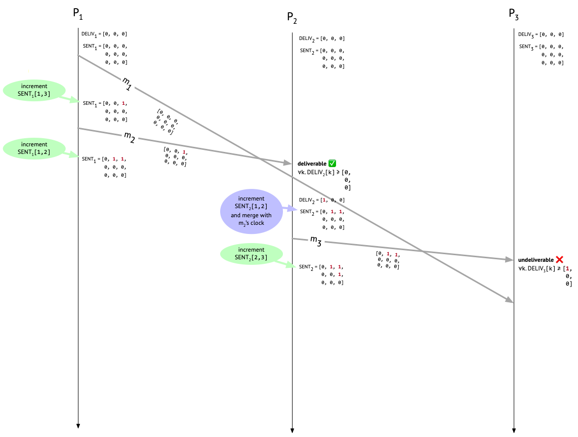
When Carol receives \(m_3\), we check if it’s deliverable by comparing the third column of the metadata attached to \(m_3\) with \(\mathit{DELIV}_3\). Since Carol hasn’t delivered any messages yet, \(\mathit{DELIV}_3\) is all zeroes. But \(m_3\)’s metadata has an entry of 1 at position [1, 3]! That tells us that \(P_2\) “knew about” one message, sent by \(P_1\) and destined for \(P_3\), at the time that \(m_3\) was sent, but that one message – \(m_1\) – hasn’t shown up yet (or it would have been recorded in \(\mathit{DELIV}_3\). Therefore, \(m_3\) is undeliverable, and must sit in the mail room.

Sorry, m_3.

But then \(m_1\) shows up at \(P_3\). We check the third column of its causal metadata and see that it’s deliverable. Hooray! \(P_3\) now increments the first entry in \(\mathit{DELIV}_3\) to show that \(P_3\) has delivered a message from \(P_1\). \(P_3\) also increments \(\mathit{SENT}_{3}[1, 3]\) to record the fact that \(m_1\) was sent by \(P_1\). The last step is to update every entry in \(\mathit{SENT}_3\) to the maximum of itself and the corresponding entry in the causal metadata attached to \(m_1\), but since \(m_1\) had no preceding messages, its causal metadata is all zeroes, so this last step is a no-op.

P_3 has delivered m_1 and updated its local state accordingly.

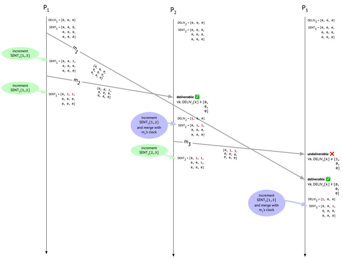
Finally, now that \(m_1\) has been delivered at \(P_3\) and \(\mathit{SENT}_{3}[1, 3]\) has been incremented, Bob’s fateful message to Carol that’s been languishing in the mail room, \(m_3\), has become deliverable. So let’s deliver it and once again update \(\mathit{DELIV}_3\) and \(\mathit{SENT}_{3}\) accordingly:

P_3 has delivered m_3 and updated its local state accordingly.

What are we left with now? \(P_2\) and \(P_3\) agree in their knowledge of how many messages have been sent, from whom they were sent, and to whom they were sent. In particular, they both know that one message was sent from \(P_1\) to \(P_2\), one message was sent from \(P_1\) to \(P_3\), and one message was sent from \(P_2\) to \(P_3\). We can see that they both know these things, because they both have the same \(\mathit{SENT}\) matrix:

[0, 1, 1,
 0, 0, 1,
 0, 0, 0]

Meanwhile, \(P_1\) is ignorant of the message that was sent from \(P_2\) to \(P_3\), and so at the end of the execution, its \(\mathit{SENT}\) matrix just looks like this:

[0, 1, 1,
 0, 0, 0,
 0, 0, 0]

Had all the messages been broadcast messages, then we wouldn’t see this; everyone’s \(\mathit{SENT}\) matrices would agree at the end of the execution. (But also, had all the messages been broadcast messages, we wouldn’t need to be using matrices anyway.)

Because the only part of the causal metadata matrix that gets checked during the deliverability check is the particular column that’s relevant to the receiver, one might ask if it’s really necessary to send the whole matrix. Couldn’t you just send the one column you’re actually going to look at, and save space? It’s true that for the metadata check, you only need one column, but the rest of the causal metadata is necessary so that the receiving process can update its \(\mathit{SENT}\) matrix appropriately and then have the most up-to-date causal metadata to attach to its own outgoing messages later. For example, \(m_2\) carries knowledge of \(m_1\) in its causal metadata. The recipient of \(m_2\), \(P_2\), does not itself care about \(m_1\). But it does want its own outgoing messages later on, namely \(m_3\), to carry knowledge of \(m_1\) too, because the recipient of those messages – in this case, \(P_3\) – might care about \(m_1\). That’s exactly what we see happening in this execution: \(P_2\) is passing along knowledge about \(m_1\) in the causal metadata attached to \(m_3\), so that \(P_3\) can make an informed decision about what to do with \(m_3\). If \(P_1\) happened to know that \(P_2\) is never going to send any messages, then it could get away with not sending this extraneous information. Other such optimizations seem possible, too.

Question: Is \(\mathit{DELIV}\) redundant?

My student Jonathan Castello observed that the \(\mathit{DELIV}_i\) data structure at each \(P_i\) seems to be redundant with the \(i\) column of \(\mathit{SENT}_i\) (that is, the column recording \(P_i\)’s knowledge of messages sent to it).

The \(\mathit{DELIV}\) vector and the \(\mathit{SENT}\) matrix serve different purposes. Your \(\mathit{DELIV}\) vector tracks how many messages you’ve delivered from everyone else, while your column of your \(\mathit{SENT}\) matrix tracks how many messages everyone else has sent to you, regardless of whether you’ve delivered them. But, would there be times when your \(\mathit{SENT}\) matrix would have knowledge of a message \(m\) being sent to you that you haven’t delivered yet? If you haven’t delivered \(m\), then you must have learned secondhand of \(m\)’s existence, via some other message \(m'\). But in that case, you wouldn’t have delivered \(m'\), because \(m\) would causally precede \(m'\)! So it would seem that for all \(i\), \(\mathit{DELIV}_i\) and \(\mathit{SENT}_i[-, i]\) will always agree with each other, in which case it seems like we could do away with the \(\mathit{DELIV}\) vectors entirely. I’d love for someone to either confirm that this is the case, or explain why it’s not. I hope my brilliant readers will weigh in here.

Discussion

One thing that’s interesting to me about Raynal et al.’s protocol is that the increment to \(\mathit{SENT}\) happens after sending the message, rather than before. This means that there’s more bookkeeping to do on the receiving end after delivering a message – both the sender and the recipient have to increment the appropriate entry in \(\mathit{SENT}\). It duplicates work! On the other hand, it simplifies the deliverability condition. If we incremented before sending a message from \(P_j\) to \(P_i\), then \(P_i\) would have to check that \(SENT_{j}[j, i]\) (the number of messages sent from \(P_j\) to \(P_i\)) was exactly one greater than \(\mathit{DELIV}_{i}[j]\) (the number of messages from \(P_j\) that \(P_i\) has already delivered). In fact, Birman et al.’s CBCAST protocol has to do exactly this kind of “one greater” check for the sender in its own deliverability condition, although in the context of broadcast rather than unicast. In Raynal et al.’s protocol, the deliverability condition doesn’t need to special-case the sender in this way. But I have a hunch that you could also implement a version of Raynal et al.’s protocol that increments before sending, adds the “one greater” clause to the deliverability condition, and drops step 2 from the post-delivery steps.

Making sure that the appropriate bookkeeping happens on both ends, and that the deliverability condition matches it, seems quite fiddly and error-prone. The pieces of the protocol have to match up; they can’t be said to be correct or incorrect in isolation, which makes bugs harder to find. I wonder if something like typed choreographies would help eliminate these kinds of bugs. More generally, I want tools that could help us safely explore the protocol design space. For this particular protocol, one trade-off seems to be: either duplicate work, or make the deliverability condition more complicated. What other knobs are there?

Thanks to Aditya Athalye and Jonathan Castello for discussing the ideas in this post with me and giving feedback on drafts.

1. Using the causal broadcast protocol in our non-broadcast setting actually wouldn’t pose any problem for safety – after all, a unicast message is just a broadcast message that’s partway through being sent! – but it would certainly be a big problem for liveness. ↩

2. When I first saw \(\mathit{SENT}\), I was under the impression that it was a two-dimensional matrix clock. A matrix clock is a generalization of a vector clock that captures “higher-order” information about the states of processes. For example, in our setup with Alice, Bob, and Carol, if a vector clock tracks what Alice knows about every participant’s state, then the corresponding two-dimensional matrix clock would also track what Alice knows about what Bob knows about every participant’s state, and what Alice knows about what Carol knows about every participant’s state. That’s not what’s going on here. Instead, the second dimension of the matrix is just being used to track destination information. So these matrices probably shouldn’t be called “matrix clocks”, although they’re certainly matrices and they’re certainly some kind of logical clock! ↩