State is Progressive, or: hey, what happens if we make literally everything append-only?
by Sohum Banerjea ⋅ edited by Natasha Mittal and Lindsey Kuper
State is weird.
State is weird because we want the freedom to mutate and mangle it however we like. That’s the default conceptualisation we have of state, since we all learnt to program – state is a bag of bits, or structs, or objects, that we can mangle however we like.
But we keep finding situations in which this view of state loses us verifiability, or reproducibility, or, god forbid, performance. Whether it’s multicore processors or distributed systems, storage systems or language models, we keep finding ourselves in cases where the bag-of-bits model lets us do less than we could.
In the effort to do more, there’s a common thread: designs that don’t mutate state, only add to it; that conceptualise knowledge as something that only monotonically grows, and never decreases.
In this post, we’ll look at a few examples of these “progressive systems”. For our purposes, it’s easiest to discuss them in terms of the axis along which they restrict state to be monotonic. Treating the data itself as always monotonic, independent of time, gets you lattice models, whereas treating time as the property that is always monotonic gives you stream models.
Lattice Models
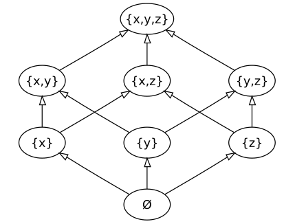
Placing this monotonicity guarantee on your data means ensuring that “bigger” data is always closer to the final state, for some definition of “bigger”. Mathematically, enforcing this structure on data cashes out to structuring it as a join-semilattice, which we obviously have to shorten to “lattice”. A join-semilattice is a set with an associated partial order, and where every pair of elements have a least upper bound (“join”) that respects that partial order. The archetypical example here is sets under the subset partial order. Every pair of sets has a least upper bound — the union of those two sets — that respects subset inclusion as a partial order. Thus, sets, under the partial order of subset inclusion and the join operation of union, form a join-semilattice.
Okay. So we can think of the states our data can take on as members of a join-semilattice. What does this actually buy us?
It means that if we have conflicting copies of our data ({2,3} and {3,5}, let’s say) at any point,
we know what to do to resolve the conflict: take the least upper bound ({2,3,5}). Since
we know our data can never get “smaller”, this is a correct operation — the state of our
data is at least what it is at each replica. This is the fundamental idea that links the following three distinct approaches to state.
CRDTs
CRDTs, or conflict-free replicated data types, try to present the concept of join-semilattices to the programmer as transparently as possible. They’re data structures designed for replication, and a lot of their complexity comes from providing expressive, efficient data structures while maintaining the property that the data is always monotonically growing. Research in the field tries hard to make the resulting data structures efficiently support the operations we want them to.
There ends up being a lot of subtlety in how more complex operations can be supported when we try to represent a data structure as a lattice — even the canonical CRDT, the set, gets complicated once we dare to do anything as gauche as deleting elements. (In short: deleting elements from a set is a non-growing operation, and so if we’re not careful, when we delete an element from one replica, the rest of our replicas will just assume it’s an addition we haven’t seen yet, and add it right back again.)
A major issue with using CRDTs in practice is how they need to be garbage collected — as you may imagine, having your state grow without bound is not a desirable property for a data structure. This is an instance of non-monotonicity in our programs: as much as we’d like our programs to be monotonic, we end up needing these synchronisation points for real-world practical usage.
LVars
LVars are another data structure that associates states with lattice elements. Any write to an LVar updates it to the least upper bound of the value being written and the state the LVar already had. Where they differ from CRDTs is in the additional restrictions they impose on how this data can be interacted with: LVars are not directly readable. The read operation on an LVar is a “threshold read” — an operation that blocks until one of a set of specified points in the lattice has been reached or surpassed, and thus can never return any intermediate state. To preserve determinism, this threshold read doesn’t even necessarily return the current state of the LVar when it unblocks. Rather, it deterministically returns a state that the current state is guaranteed to be at or above.
In exchange, LVars recover determinism. That is, all interleavings of a program that coordinates data with LVars will produce the same result. This design decision is a more natural set of tradeoffs to want in their domain: LVars were designed for shared memory, whereas CRDTs were designed for replicated data.
There is a way to read the exact state of the LVar, but only after it’s been “frozen”. This creates the opportunity for races between attempts to write to the LVar and attempts to freeze it, and thus this weakens the determinism guarantee to “quasi-determinism” — all interleavings of the program are guaranteed to produce the same result as long as that interleaving doesn’t error.
LVars don’t aim to adddress non-monotonic use cases; instead, the philosophy is that they can just give up control over the data once a non-monotonic operation is necessary. The assumption is that a non-monotonic operation will not be necessary until after a (often lengthy) phase of monotonic computation, and so LVars allow parallelisation of the monotonic phase.
Bloom and Bloom^L
Bloom and its successor Bloom^L build monotonicity right into a programming language – or, to be more precise, they remove operations until the only operations left are monotonic.
The idea is that non-monotonicity is what leads to the need for synchronisation in distributed programs. If your program is not monotone, then it will need to have all of its inputs to produce the correct result. Some approaches to distributed programming weaken the “correctness” of the result in response, but if you could program with purely monotonic operations most of the time, you could narrow down the places you need to synchronise to those places where you’re using non-monotonic operations. This is the CALM principle — “Consistency As Logical Monotonicity”.
Bloom^L has you write monotone functions on data structures, so it can
ensure that the entire program’s use of state is monotone and thus doesn’t need
synchronisation to ensure eventual consistency.
One particularly useful class of monotone functions is homomorphic functions — functions that map from one lattice to another, ensuring the map
preserves the structure of the lattice while doing so.
For instance, under the standard lattice for sets, a set.is_empty() operation is
homomorphic if and only if the resulting boolean is false-biasing. That is, false > true
in its lattice, and thus ifnot is the only monotonic operation available on it, not if.
The constraints of Bloom^L allow it to guarantee monotonicity without static checking in most cases.
(Psst. Don’t tell anyone, but Bloom^L also belongs in the next section. See you there!)
Data as Streams
Another way to have grow-only state is to just totally order it in time. Despite all the problems in trying to totally order time, there are some cases in which we can structure the entirety of how we process state such that we can exploit this total ordering.
In practice, these designs look like stream processing languages. Streams are inherently ordered
data, which means we always know what’s newer and what’s older, and stream processing is
inherently an operation in time, such that any stream processor can only ever emit at time
t data that is dependent on input data up to time t. This is, of course, monotonicity
again, just pushed a layer outward, into metadata — timestamps — associated with our data cells.
In this framework, one key requirement keeps showing up: for the system or a stream to
somehow guarantee that no further messages with timestamps ≤ t will appear. Most
commonly referred to as “punctuation”, this shows us the key point at which we
fundamentally need to guarantee the (local) monotonicity of time for our operations on
these streams to continue being monotonic.
CQL
CQL, the “Continuous Query Language”, takes this framing and applies the well-known declarative language of relational logic (i.e., SQL) to streams.
The core of CQL is in its stream-to-relation and relation-to-stream operators, in order to let the standard SQL operators do work on the intermediate relations. It deliberately does not provide stream-to-stream operators, requiring all operations to be done on the relational layer. To do this, they augment their concept of relations to natively include time; all relations in CQL are time-varying (parameterised by timestamp).
Both of these classes of operators are simple to specify:
- stream-to-relation operators capture a given time window over the stream and present the data within that window as a relation with the same schema
- relation-to-stream operators emit elements on the stream at time
twhen- an element is added to the relation at time
t(Istream) - an element is deleted from the relation at time
t(Dstream) - or, an element just is in the relation at time
t(Rstream)
- an element is added to the relation at time
The language attempts to add a default Istream in cases where a conservative static
check of the underlying relation can guarantee that the relational operation being
described is monotonic.
Punctuation isn’t considered a language-level concern for CQL — the language assumes you
have access to all data up to timestamp t when computing something at timestamp t, and
it’s left to the runtime to validate this requirement. However, they do describe that
their runtime does need to have ways of generating these “heartbeats”, and various
policies for doing so.
Bloom^L
Bloom^L also uses streams as a core data type. More precisely, it parameterises its data cells by time, thus providing a similar set of properties to stream based languages. It does this in order to model the nondeterminism of asynchronous communication (a message from one node to another is modelled as data inserted into a shared object at a nondeterministic future timestamp).
Bloom^L is capable of reasoning about non-monotone parts of your program, and this integration of time into its modelling is a major reason why it can do so.
When you allow Bloom^L to reason about punctuation, you get Edelweiss, a generic solution to the garbage collection problem CRDTs have to face. Edelweiss has a far more general concept of punctuation than either other system — it’s a guarantee that no more messages will arrive matching any arbitrary predicate. Edelweiss can then track these predicates across channels compositionally (if the set of peers at a particular epoch is fixed, and all of those peers have responded to a given message, it’s guaranteed that one will not receive any further responses to that message).
Pervasive monotonicity, combined with the strong guarantees Edelweiss enables via its punctuation system, allow the user to reason directly about what state they no longer need to keep around and can thus garbage-collect.
Timely Dataflow
Timely dataflow is an approach to stream processing that has handling of iterative loops as an explicit design goal. Loops are constrained specifically to ensure they manage the timestamps of messages flowing through the system in a precise, predictable, monotonic way.
Since the system has more control over the timestamps than a general stream processing system, it can reason about how messages could result in later messages at given timestamps — essentially providing a flexible, productive method for generating punctuation across the whole system in the presence of loops. This allows for complex dataflows across the resulting stream processing nodes, including messages sent to nodes at specific future timestamps, and nodes that wait for punctuation before computing some non-incremental property of the data.
Again, we find monotonicity, as modified to address the problem, to provide strong properties we can exploit — even when computing non-monotonic properties.
What Does All This Mean?
State is progressive.
…Okay, that may be overselling it. While all of these models have important benefits when applied to the use cases they were designed for, none of them attempt to be a general-purpose model of state. We’re not yet trying to overthrow the von Neumann machine as the fundamental architecture on which computation is built.
That said, these designs do point to a “turning point” in how we think about state. If you can stomach the limitations of designing your state to be progressive, you get strong, relevant properties in return.
State may be progressive. Maybe it’s time to seriously consider those designs.